Home
Course Guidelines
About the course Prerequite Material References
Python
Jupyter Notebooks Python overview
Exercises
Before the semester start: Installation and exercise setup Week 1: Introduction to Python and libraries Week 2: Vector representations Week 3: Linear Algebra Week 4: Linear Transformations Week 5: Models and least squares Week 6: Assignment 1 - Gaze Estimation Week 7: Model selection and descriptive statistics Week 8: Filtering Week 9: Classification Week 10: Evaluation Week 11: Dimensionality reduction Week 12: Clustering and refresh on gradients Week 13: Neural Networks Week 14: Convolutional Neural Networks (CNN's)
Tutorials
Week 1: Data analysis, manipulation and plotting Week 2: Linear algebra Week 3: Transformations tutorial Week 4: Projection and Least Squares tutorial Week 7: Cross-validation and descriptive statistics tutorial Week 8: Filtering tutorial Week 11: Gradient Descent / Ascent
In-class Exercises
In-class 1 In-class 2 In-class 10 In-class 3 In-class 4 In-class 8
Explorer

Document

  • Overview
  • 1. Data preprocessing and eye feature extraction
  • 2. Assignment: Gaze estimation

Content

  • Gaze Estimation introduction
    • Gaze mapping function
  • Gaze estimation test subject 0
    • Data and visualization
      • Task 1 Data visualization
  • Implement a gaze estimation model
    • Task 2 Initial reflection
    • Task 3 Implement a gaze model
    • Task 4 Model evaluation
    • Task 5 Visualize performance of your model
    • Task 6 Evaluate performance of your model
  • Test on test subject 3
    • Task 7 Load the data
    • Task 8 Visualize performance
    • Task 9 Evaluation
  • Gaze estimation test subject 3
    • Task 10 Train and test a model
    • Task 11 Evaluation
    • Task 12 Evaluation(continued)
    • Task 13 Evaluation(continued)
    • Task 14 Evaluation(continued)
    • Task 15 Adding more data
    • Task 16 Evaluate
  • Individual dataset
    • Task 17 Individual dataset
    • Task 18 Train and test a model
    • Task 19 Evaluate
  • Task 20 Explore your dataset
  • Scale the data
    • Task 21 Scale the data
    • Task 22 Evaluation
  • Improve the model
    • Task 23 Model improvements
    • Task 24 Evaluation

Assignment introduction

Overview

This is the first mandatory assignment in which you will implement a regression model to estimate where a person is looking (this is known as gaze) from images of eyes.

You only have to hand in this Jupyter Notebook containing your implementation and notes (markdown or python cells), see the bottom of this page for handin details. For the TA's to assess the assignment we kindly ask you to also hand in the data folder. If you are not comfortable sharing your data with the TA's leave that folder out for the handin, but provide the plots for assessment. Refer to the bottom of the page for submission details.

Before you start solving the assignment, carefully read through the entire assignment to get an overview of the problem and the tasks.

Notice that the optional Task 23 and onward relates to exercises in next week. You may save some time by postponing it until then.

Important! Complete all tasks marked with high (red) priority before attempting to solve the others, as they are optional. Optional tasks and further analysis can help improve results, but feel free to explore methods and data as you choose.
The assignment builds on the Data preprocessing exercise using the data in the data folder as well as your own. You will start with the data of test_subject_0 . You will then try out the model using the data from the data collection session.

The assignment is structured in the following way:

  • Train gaze estimation models using data from test_subject_0 training set.
    • Test the models using test_subject_0 test set.
    • Test the models using test_subject_3 .
  • Train gaze estimation models using data from test_subject_3 , grid .
    • Test the models using test_subject_3 .
  • Train gaze estimtion models using your own data set.
Note

The assignment has multiple steps, but the procedures will repeat. Duplicate code as needed to keep results in each cell, making it easier to review during the exam.

To simplify the assignment, most visualization and data processing code is in iml_util.py . You can review it, but you're not expected to explain it. Focus on the code provided in the assignment.

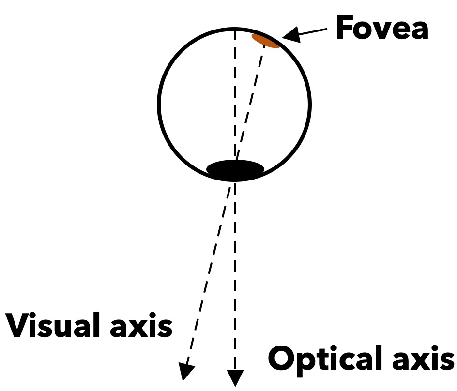
The location of the fovea on the retina varies between people ($\pm$ 5 degrees). Consequently, a gaze model has to be trained (calibrated) for a specific person to be accurate. This difference is shown in Figure 1.

Gaze Estimation introduction

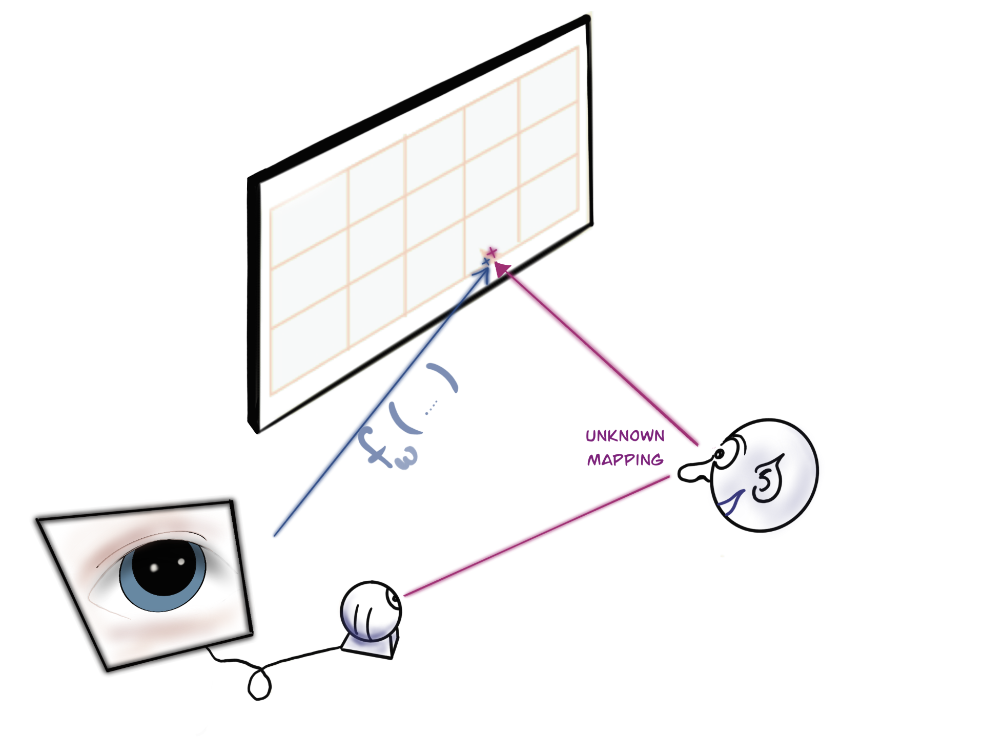
Gaze estimation is performed by capturing images of a user's eye as shown in Figure 2 and mapping them to screen positions using a function $f_\mathbf{w}(x, y)$. Humans look at things by orienting their eyes so that the light from the point of focus hits the Fovea (a point on the retina). The Fovea is not directly aligned with the center of the pupil, but at a person-specific angle, as shown in Figure 1. The pupil position can be used to infer gaze, but to obtain accurate gaze estimates requires training data (called calibration).

Figure 1:

The distinction between the visual and optical axes. The optical axis is defined as an axis perpendicular to the lens behind the pupil. The visual axis depends on the placement of the fovea.

Figure 2:

Diagram of a gaze estimation system. The eye, which is directed at a specific point on the screen is captured by the camera. The two red lines represent an unknown transformation from image to eye and eye to screen. We learn this transformation directly which is shown as $f_{\mathbf{w} }(x, y)$ in the diagram.

Gaze mapping function

The goal of this exercise is to estimate gaze from image sequences using a regression model. Define $f_{\mathbf{w}}(x, y)$ as the gaze model which maps pupil positions $(x, y)$ to screen coordinates $(x', y')$. The model parameters $\mathbf{w}$ are learned from a training set containing paired pupil and screen positions.

Gaze estimation test subject 0

The first step is to train a gaze estimation model using the dataset of test_person_0 . You will:

  • Train the models using the data pupils_n_training and screen_coordinates_training .
  • Test the performance of the model using the pupils_n_testing and screen_coordinates_testing .

Data and visualization

Task 1: Data visualization
  1. Inspect the structure of the dataset by revisiting exercise Data preprocessing section Visualization.
  2. Run the cell below to visualize the data of test_subject_0 .
import os import numpy as np import matplotlib.pyplot as plt import iml_util D = iml_util.gen_data_subject_0() for i in range(4): dataset = D[i] grid = iml_util.create_image_grid_viz(dataset) iml_util.image_and_scatter(grid, dataset)
import os
import numpy as np
import matplotlib.pyplot as plt
import iml_util

D = iml_util.gen_data_subject_0()
for i in range(4):
    dataset = D[i]
    grid = iml_util.create_image_grid_viz(dataset)
    iml_util.image_and_scatter(grid, dataset)

Implement a gaze estimation model

Figure 3:

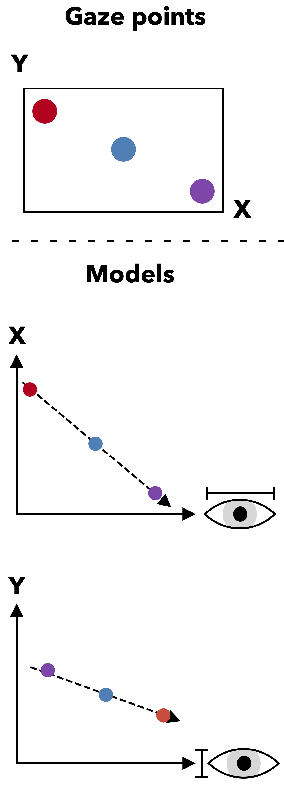
Point mapping. Top: Three screen coordinates. Middle: Screen and eye $x$ coordinates for the same three points. Bottom: Screen and eye $y$ coordinates for the same three points.

The true nature of the function that transforms pupil positions to screen positions is not easy to model. Even when the head is stationary, the relationship between pupil position in the image and gaze is non-linear due to the pupil's movement along a spherical curve. For now, we'll approximate the gaze mapping by using a linear function.

Since the goal is to predict a $2D$ screen coordinate from a $2D$ pupil coordinate, it's more straightforward to train two separate models for each coordinate by following the pattern of previous exercises. The linear gaze model can be expressed as:struct

$$ \begin{aligned} x' &= ax + by + c\\ y' &= dx + ey + f. \end{aligned} $$

Gaze mappings is demonstrated in Figure 3 to the right. Here, the $x$ coordinate of the pupil maps to the $x$ coordinate on the screen. In the real model, we use both $x$ and $y$ as inputs to both models estimating the $x$ position and $y$ position on the screen.

Hint

Use the previous exercise as a guideline.

In the upcoming tasks, you will be guided through the process of identifying essential entities necessary for establishing the linear equations required to learn the model parameters of the given model. The gaze model is divided into two distinct regression models, denoted as $x' = f_{w_1}(x, y)$ and $y' = f_{w_2}(x, y)$, each associated with its unique set of model parameters $w_1$ and $w_2$. Essentially, one model predicts the value of $x'$, and the other model predicts the value of $y'$. Follow the steps outlined below for the model $x' = f_{w_1}(x, y) = ax + by + c$, and subsequently, replicate the same steps for $y'$.

  1. Identify model parameters and inputs to the model. We recommended that you use Least Squares from the numpy library linalg.lstsq , it is recommended due to numerical stability.
  2. Isolate the unknown model parameters and the known into the design matrix.
  3. Setup the linear equations $Aw=b$, where $A$ is the design matrix, $w$ the unknown model parameters and $b$ contains labels.
Task 2: Initial reflection
  1. Identify the model parameters, inputs and outputs for the model.
  2. Identify and determine the minimim number of data points needed to fit the model.
  3. Using the least amount of points required to fit the model, does it matter which points are used? Why? Why not?
#Write your reflection here...
Task 3: Implement a gaze model

You can choose to train two separate models, to predict each screen coordinate separately, or you can train one model predicting both coordinates simultaniously. It may be slightly simpler to use two separate models.

  1. Design matrix: Implement a function get_design_matrix to create the design matrix from an array pupil positions.

  2. Calibration: Complete the implementation of the function calibrate of the class LinearGaze .

    • Use the pupils_n_train and screen_coordinates_train arrays as training data.
    • Use the function get_design_matrix to create a design matrix from the pupil positions.
    • Learn the parameters $\mathbf{w}$ from the dataset using Least Squares.
  3. Gaze estimation: Finish the implementation of the function predict of the class LinearGaze which predicts the gaze point given a pupil position using the learned model parameters. For reference, the affine model has the form $f_\mathbf{w}(x)=\mathbf{w}_0 x_0 + \mathbf{w}_1 x_1 + \mathbf{w}_2$. You may calculate the point for each coordinate seperately. Return the estimated screen coordinates using the models created during calibration.

Important! Don't expect the affine model to perform particularly well. Expect the distances between true and predicted gaze points to vary by $\pm 200$ pixels.

def get_design_matrix(pupil_positions): """ Constructs a design matrix. Parameters: pupil_positions (N x 2 numpy array): n samples, 2 features (px, py). Returns: design_matrix (N x 3 numpy array) : n_samples, 2 features + 1 """ # Write your implementation def linear(param, x): return param[0] + param[1]*x[0] + param[2]*x[1] class GazeModel: def calibrate(self, dataset): ... def predict(self, pupil): ... def predict_many(self, pupils): return np.array([self.predict(pupil) for pupil in pupils]) class LinearGaze(GazeModel): def calibrate(self, dataset, pupil_training_set, screen_training_set): """ Calibrates the LinearGaze model by fitting two linear regression models for x and y coordinates based on the training dataset. Parameters: dataset (dict): The dictionary D containing the training data with two keys: - "pupils_train" (N x 2 numpy array): n samples, 2 features (px, py) representing pupil positions. - "positions_train" (N x 2 numpy array): n samples, 2 features (screen coordinate x, screen coordinates y) representing the true gaze positions being the screen coordinates. Returns: None: Updates the model's parameters (self.model_x, self.model_y) based on the least squares solution for x and y positions. """ # Write your implementation def predict(self, pupil): """ Predicts the gaze position (x, y) based on the given pupil position using the calibrated model. Parameters: pupil (1 x 2 numpy array): 2 features (px, py) representing the current pupil position. Returns: x, y (float, float): Predicted gaze position (x, y) based on the linear model. """ # Write your implementation
def get_design_matrix(pupil_positions):
    """
    Constructs a design matrix.
    Parameters:
    pupil_positions (N x 2 numpy array): n samples, 2 features (px, py).
    
    Returns:
    design_matrix (N x 3 numpy array) : n_samples, 2 features + 1
    """
    # Write your implementation

def linear(param, x):
    return param[0] + param[1]*x[0] + param[2]*x[1]

class GazeModel:
    def calibrate(self, dataset):
        ...

    def predict(self, pupil):
        ...

    def predict_many(self, pupils):
        return np.array([self.predict(pupil) for pupil in pupils])


class LinearGaze(GazeModel):
    def calibrate(self, dataset, pupil_training_set, screen_training_set):
        """
        Calibrates the LinearGaze model by fitting two linear regression models for x and y coordinates based 
        on the training dataset.

        Parameters:
            dataset (dict): The dictionary D containing the training data with two keys:
                - "pupils_train" (N x 2 numpy array): n samples, 2 features (px, py) representing pupil 
                  positions.
                - "positions_train" (N x 2 numpy array): n samples, 2 features (screen coordinate x, screen coordinates y) representing
                  the true gaze positions being the screen coordinates.

        Returns:
            None: Updates the model's parameters (self.model_x, self.model_y) based on 
            the least squares solution for x and y positions.
        """
        # Write your implementation


    def predict(self, pupil):
        """
        Predicts the gaze position (x, y) based on the given pupil position using the calibrated model.

        Parameters:
            pupil (1 x 2 numpy array): 2 features (px, py) representing the current pupil position.

        Returns:
            x, y (float, float): Predicted gaze position (x, y) based on the linear model.
        """
        # Write your implementation
Task 4: Model evaluation

The following task is about evaluating the performance of your models. In the following task you will complete the function results_for_model . It is important that the results are calculated for the complete dataset of test_subject_0 (all of $\mathcal{D}_{p0}, \mathcal{D}_{p1}, \mathcal{D}_{p2}, \mathcal{D}_{p3}$ as one dataset).

  1. Finish the implementation of the function results_for_model . For each dataset it must:
    • Calculate prediction errors:
      • Calculate:
        • The absolute error between each prediction and true gaze.
        • The mean Eucledian distance between the true values and the predictions.
        • The root-mean-square error (rmse) between the true values and the predictions.
        • The mean absolute error (mae) as well.
def results_for_model(model, dataset_train, dataset_test, pupil_training_set, screen_training_set, pupil_test_set, screen_test_set, d_max): """ Evaluates the performance of the model across multiple datasets and computes prediction errors. Parameters: model (object): A gaze model object. d_max (int, optional): Maximum number of patterns of a dataset to evaluate. Default is 4. Returns: results (dict): A dictionary where each key corresponds to a dataset index (0 to d_max-1), and each value is a dictionary containing: - "predicted" (1 x N numpy array): The predicted values - "ground_truth" (1 x N numpy array): The corresponding ground truth values to the predicted - "model_x" (list): List of model paramters for model x - "model_y" (list): List of model paramters for model y - "errors" (N x 2 numpy array): Absolute errors between predicted and ground truth positions (x, y). - "rmse" (float): Root Mean Squared Error (RMSE) for the predictions across the dataset. - "dist" (float): Mean Euclidean distance between the predicted and actual positions. - "mae" (1 x 2 numpy array): Mean absolute error in x and y dimensions. """ results = {} for d in range(d_max): train = dataset_train[d] test = dataset_test[d] model_x, model_y = model.calibrate(train, pupil_training_set, screen_training_set) predicted = model.predict_many(test[pupil_test_set]) ground_truth = test[screen_test_set] # Write your solution here return results return results results_linear = results_for_model(LinearGaze(), D, D, 'pupils_n_train', 'screen_coordinates_train', 'pupils_n_test', 'screen_coordinates_test', 4)
def results_for_model(model, dataset_train, dataset_test, pupil_training_set, screen_training_set, pupil_test_set, screen_test_set, d_max):
    """
    Evaluates the performance of the model across multiple datasets and computes prediction errors.

    Parameters:
        model (object): A gaze model object.
        d_max (int, optional): Maximum number of patterns of a dataset to evaluate. Default is 4.

    Returns:
        results (dict): A dictionary where each key corresponds to a dataset index (0 to d_max-1), and each value is a dictionary containing:
            - "predicted" (1 x N numpy array): The predicted values
            - "ground_truth" (1 x N numpy array): The corresponding ground truth values to the predicted
            - "model_x" (list): List of model paramters for model x 
            - "model_y" (list): List of model paramters for model y 
            - "errors" (N x 2 numpy array): Absolute errors between predicted and ground truth positions (x, y).
            - "rmse" (float): Root Mean Squared Error (RMSE) for the predictions across the dataset.
            - "dist" (float): Mean Euclidean distance between the predicted and actual positions.
            - "mae" (1 x 2 numpy array): Mean absolute error in x and y dimensions.
    """


    results = {}
    for d in range(d_max):
        train = dataset_train[d]
        test = dataset_test[d]
        model_x, model_y = model.calibrate(train, pupil_training_set, screen_training_set)
        predicted = model.predict_many(test[pupil_test_set])
        ground_truth = test[screen_test_set]
    # Write your solution here
    return results
return results


results_linear = results_for_model(LinearGaze(), D, D,  'pupils_n_train', 'screen_coordinates_train', 'pupils_n_test', 'screen_coordinates_test', 4)

Below you find a cell containing a function for visualizing the performance of the model.

Task 5: Visualize performance of your model
  1. Create visualizations: Run the cell below to visualiz the performance of the model for all patterns using the function plot_results_grid from iml_util.py . The function takes a dictionary of results as well as the number of patterns in the dictionary. Combined they provide an overview of the nature of the error across the two dimensions.
iml_util.plot_results_grid(results_linear, 4)
Task 6: Evaluate performance of your model
  1. Evaluate the usefulness of the mae or rmse and their differences.
  2. Identify at least 3 potential sources of error associated with the current affine model. Describe how each source of error contributes to the prediction error.
#Write your reflection here...

You have now went through the first part of the assignment processing the session of test_subject_0 . The remaining part of the assignment use the same approach as you have just gone through with the purpose of you working with and reflecting on the use of your own data collected.

Test on test subject 3

In the data processing exercise Data preprocessing the pupil corrdinates mean_pupil_coordinates.csv and the corresponding screen coordinates screen_coordinates.csv were saved in the in the folder with the test subjects and patterns. Recall the four calibration patterns used for the data collection being grid, circle, line and random.

In this exercise you will use the calibration (training data) of test_subject_0 on the data from test_subject_3 and visualized in Figure 4.

Figure 4: Left: Images fron calibration pattern grid. Middle: Calibration pattern. Right: Pupil center scatterplot from calibration pattern grid.
Task 7: Load the data
  1. Run the cell below to load the data of test_subject_3 . Similarily to the data of test_subject_0 meaning that the grid pattern is defined as training set for all other patterns. The data is stored as a list of dictionaries in the following order: grid , circle , line , and random . Within each dictionary you find:
Details about the data format of `test_subject_3`

Dataset elements:

  • pupils_train : Mean pupil positions for the 9 calibration points from grid pattern (an $9 \times 2$ array containing the x and y coordinates (px , py )).
  • screen_coordinates_train : Screen target positions for the 9 calibration points from grid pattern ($9 \times 2$ array containing x,y pixel position for the target on the screen (sx , sy )).
  • pupils_test : Mean pupil positions for the calibration points for the pattern accociated as the key(an $N \times 2$ array containing the $N$ x and y coordinates (px , py )).
  • screen_coordinates_train : Screen target positions for the N calibration points associated to the pattern defined as the key ($N \times 2$ array containing the $N$ x andy pixel positions for the target on the screen (sx , sy ))
D3 = iml_util.gen_data_subject('test_subject_3')
Task 8: Visualize performance
  1. Run the cell below to evaluate the gaze estimation model using the data from test_subject_3
results_linear_ts3 = results_for_model(LinearGaze(), D, D3, 'pupils_n_train', 'screen_coordinates_train', 'pupils_test', 'screen_coordinates_test', 4) iml_util.plot_results_grid(results_linear_ts3, 4)
results_linear_ts3 = results_for_model(LinearGaze(), D, D3, 'pupils_n_train', 'screen_coordinates_train', 'pupils_test', 'screen_coordinates_test', 4)

iml_util.plot_results_grid(results_linear_ts3, 4)
Task 9: Evaluation

You likely have observed larger prediction errors, including the MAE_y and RMSE . Reflect on:

  1. How well does the model predict gaze of test_subject_3 ?
  2. Use your reflections in Task 8 in the exercise Data preprocessing to elaborate on the results in this exercise.
  3. Comment on differences between the predicted x and y coordinate.
#Write your reflections here...

Gaze estimation test subject 3

In this the gaze estimation model is trained using the grid pattern of test_subject_3 , and test it on the patterns.

Task 10: Train and test a model
  1. Use result_for_model to train and test a gaze estimation model based on test_subject_3 .
  2. Use plot_results_grid to visualize the result.

The result using pupil centers from the grid pattern is a result of training and testing on the same data.

# Write your code here
Task 11: Evaluation
  1. Reflect on the result testing the model on test_subject_3 .
    • Use your reflection from Task 8 in exercise Data preprocessing to elaborate on the result.
      • Why does the performance of the model trained on test_subject_3 show significantly larger prediction errors compared to the one trained and tested on test_subject_0 ?
#Write your reflections here...

You may by now you have observed that the model is struggling with properly predicting the y coordinates. The cell below visualizes the model predictions separating the x and y coordinate.

Task 12: Evaluation(continued)
  1. Run the cell below to viualize the models independently.
  2. Use the plot for further evaluation, reflect on the questions:
    • Observe that the model are struggling the most in predicting the y coordinate correctly. What is a possible explanation for this?
    • What would happen to the plane if we train the model on more data points?

Incoorporate your reflections from exercise Data preprocessing Task 8.

for i in range(len(results_linear_ts3)): iml_util.plot_from_results_dict(results_linear_ts3[i], D3[i])
for i in range(len(results_linear_ts3)):
    iml_util.plot_from_results_dict(results_linear_ts3[i], D3[i])

To further elaborate on the prediction of the y coordinate, the cell below visualizes the Sum of Squared Error (SSE) loss function, in parameter space. The cell below creates two plots, left is the loss when changing parameters a and b while keeping c fixed. The right plot shows loss when varying c while keeping a and b fixed.

Task 13: Evaluation(continued)
  1. Run the cell below to visualize the loss described by the parameters.
  2. Describe the effect each parameter has on the SSE.
# Example usage with sample data x = D3[0]['pupils_train'][:,0] y = D3[0]['pupils_train'][:,1] z = D3[0]['screen_coordinates_train'][:,1] # Actual targets # Set fixed values for a, b, and c (based on an example linear model) a_fixed = results_linear_ts3[0]['model_y'][2] b_fixed = results_linear_ts3[0]['model_y'][1] c_fixed = results_linear_ts3[0]['model_y'][0] # Plot the error surfaces iml_util.plot_error_surfaces(a_fixed, b_fixed, c_fixed, x, y, z)
# Example usage with sample data
x = D3[0]['pupils_train'][:,0]
y = D3[0]['pupils_train'][:,1]
z = D3[0]['screen_coordinates_train'][:,1]  # Actual targets

# Set fixed values for a, b, and c (based on an example linear model)
a_fixed = results_linear_ts3[0]['model_y'][2]
b_fixed = results_linear_ts3[0]['model_y'][1]
c_fixed = results_linear_ts3[0]['model_y'][0]

# Plot the error surfaces
iml_util.plot_error_surfaces(a_fixed, b_fixed, c_fixed, x, y, z)
#Write your reflections here...
Task 14: Evaluation(continued)
  1. Observe that it appears as the prediction could benefit from a different value of c than the least square model has learned. Reflect on why this occurs.
    • Why might adjusting the slope be more important for reducing the overall error?
    • How might this affect the optimization of $c$ compared to $a$ and $b$ when there is a large scale difference between inputs and labels?

Hint: The model minimizes the total error by adjusting the parameters. Changing a and b affects how well the slope fits the data trend, while c just shifts the plane. The model tries to minimize the sum of squared errors $\sum \left( z - (ax + by + c) \right)^2$. If $x$ and $y$ are much smaller in scale than $z$, the terms $a \cdot x$ and $b \cdot y$ contribute less to the error than $c$.

#Write your reflections here...

Until now the models have been trained using the nine calibration points from the grid pattern. You will now increase the amount of training data by incoorporating all patterns except circle . The pattern circle will be used for testing. In the cell below a dictionary D3_mod contains the training and test data similar to the structure of D and D3 . .

Task 15: Adding more data
  1. Use the functionresults_for_model and the LinearGaze class to train a new model using D3_mod . Use plot_results_grid to visualize the results and the function plot_from_results_dict to visualize the models.
  2. Run the cell below to train and test the model and visualize the result.
D3_mod = {} ts3_p_train = D3[0]['pupils_test'] ts3_s_train = D3[0]['screen_coordinates_test'] ts3_p_test = D3[1]['pupils_test'] ts3_s_test = D3[1]['screen_coordinates_test'] for i in range(2,4): ts3_p_train = np.vstack((ts3_p_train,D3[i]['pupils_test'])) ts3_s_train = np.vstack((ts3_s_train,D3[i]['screen_coordinates_test'])) D3_mod['pupils_train'] = ts3_p_train D3_mod['screen_coordinates_train'] = ts3_s_train D3_mod['pupils_test'] = ts3_p_test D3_mod['screen_coordinates_test'] = ts3_s_test D3_mod = [D3_mod] # Write your code here
D3_mod = {}

ts3_p_train = D3[0]['pupils_test']
ts3_s_train = D3[0]['screen_coordinates_test'] 

ts3_p_test = D3[1]['pupils_test']
ts3_s_test = D3[1]['screen_coordinates_test']

for i in range(2,4):
    ts3_p_train = np.vstack((ts3_p_train,D3[i]['pupils_test']))
    ts3_s_train = np.vstack((ts3_s_train,D3[i]['screen_coordinates_test']))
    
D3_mod['pupils_train'] = ts3_p_train
D3_mod['screen_coordinates_train'] = ts3_s_train
D3_mod['pupils_test'] = ts3_p_test
D3_mod['screen_coordinates_test'] = ts3_s_test

D3_mod = [D3_mod]

# Write your code here
Task 16: Evaluate
  1. How does adding more training data affect the results.
    • Does increasing the amount of training data always improve the model's accuracy?
    • How does the variability in the data affect the model's ability to generalize when more data is added (elaborate on your reflection from Task 2.3)?
    • How could adding more data influence the optimization of the model parameters?
#Write your reflections here...

Individual dataset

The pipeline of collecting data, training a model, testing, and evaluating it has been introduced. In this task, the data of your eyes will be used to train a model. Use the evaluation tools introduced in the assignment.

Important! In case you do not want to share your data with the TA's for assessment, train and evaluate the models using your data and place images of the evaluation in the folder data/output/individual . Comment out the coding cells for this part of the assigment for handin to allow TA's to run the entire notebook without errors, c.f. submitting details on About the course . Submit the assignment without the data folder containing your data, and refer to evaluation images by name in your reflections.

Task 17: Individual dataset
  1. For reproduceability, write the threshold, x_margin, y_margin and side values that was used in the processing your data in Task 4 of the Data preprocessing exercise.
#Note the values here # Threshold = # x_margin = # y_margin = # side =
#Note the values here
# Threshold = 
# x_margin = 
# y_margin = 
# side =
Task 18: Train and test a model
  1. Run the cell below to generate a dictionary of your own data.
  2. Train an affine gaze estimation model using the pattern grid .
  3. Test the model on all patterns.
# update the parameter and uncomment the line below #iml_util.gen_data_subject('group-xx-xxxx')
# update the parameter and uncomment the line below
#iml_util.gen_data_subject('group-xx-xxxx')
#Use this cell to train and evaluate your model...
Task 19: Evaluate
  1. As in previous tasks, reflect on the results.
# Write your reflections here...

Optional improvements

You may experience that the models behave differently on your dataset than on test_subject_0 and test_subject_3 . This can be due to several factors, some of which you may have already reflected on in Task 8 in exercise Data preprocessing . If you experience interesting behaviour in the predictions of your model you are of course welcome to explore it further such as:

  • Different combinations of training set (use can use the creation of D3_mod for inspiration as to how to manipulate the combination of data for training and testing).
    • If you have multiple data sets in your group, you can incoorporate those or use the ones provided, test_subject_3 or test_subject_1 .
  • Other evaluation metrics
  • Take inspiration from the optional exercises below, to explore your dataset further.
Task 20: Explore your dataset
  1. Investigate your results and explore options for improving predictions and evaluation.

Scale the data

In this task, you will improve the model using normalization. In Task 13, you reflected on the effect of having a large scale difference between input and output. Use the data of test_subject_3 in dictionary D3 .

Task 21: Scale the data
  1. Complete the functions normalize and denormalize .
  2. Train and test a model using normalized data from test_subject_3 . (Note that for the grid pattern you are using the same data for testing and training).
  3. Visualize the results using the function plot_results_grid .
from sklearn.preprocessing import MinMaxScaler def normalize(data_set): """ Normalizes the pupil and screen coordinate data in the dataset using MinMaxScaler. Parameters: data_set (list of dict): A list of dictionaries where each dictionary contains training and testing data for pupils and screen coordinates. Keys include: - 'pupils_train': N x 2 array of pupil coordinates for training. - 'screen_coordinates_train': N x 2 array of screen coordinates for training. - 'pupils_test': N x 2 array of pupil coordinates for testing. - 'screen_coordinates_test': N x 2 array of screen coordinates for testing. Returns: d (list of dict): A list of dictionaries with normalized pupil and screen coordinate data. Keys include: - 'pupils_train': Normalized N x 2 array of pupil coordinates for training. - 'screen_coordinates_train': Normalized N x 2 array of screen coordinates for training. - 'pupils_test': Normalized N x 2 array of pupil coordinates for testing. - 'screen_coordinates_test': Normalized N x 2 array of screen coordinates for testing. scaler (MinMaxScaler object): The fitted MinMaxScaler object used for normalization. """ scaler = MinMaxScaler() # Write your code here def denormalize(dataset, scaler): """ Denormalizes predicted and ground truth coordinates and calculates errors and performance metrics. Parameters: dataset (list of dict): A list of dictionaries where each dictionary contains prediction results. Keys include: - 'predicted': N x 2 array of normalized predicted coordinates. - 'ground_truth': N x 2 array of normalized ground truth coordinates. scaler (MinMaxScaler object): The MinMaxScaler object used for normalization, applied here to inverse-transform data. Returns: d (dict): A dictionary where each key corresponds to a dataset index, and each value contains the following: - 'predicted': Denormalized N x 2 array of predicted coordinates. - 'ground_truth': Denormalized N x 2 array of ground truth coordinates. - 'errors': N x 2 array of absolute errors between predicted and ground truth coordinates. - 'mse' (1 x 2 numpy array): Mean squared error for the x and y coordinates. - 'rmse' (float): Root mean squared error (RMSE) across the dataset. - 'dist' (float): Mean Euclidean distance between predicted and ground truth positions. - 'mae' (1 x 2 numpy array): Mean absolute error for the x and y coordinates. """ # Write your code here # Write your code here for training, testing and visualizing results
from sklearn.preprocessing import MinMaxScaler
def normalize(data_set):
    """
    Normalizes the pupil and screen coordinate data in the dataset using MinMaxScaler.
    Parameters:
        data_set (list of dict): A list of dictionaries where each dictionary contains training and testing data 
                                 for pupils and screen coordinates. Keys include:
                                 - 'pupils_train': N x 2 array of pupil coordinates for training.
                                 - 'screen_coordinates_train': N x 2 array of screen coordinates for training.
                                 - 'pupils_test': N x 2 array of pupil coordinates for testing.
                                 - 'screen_coordinates_test': N x 2 array of screen coordinates for testing. 
    Returns:
        d (list of dict): A list of dictionaries with normalized pupil and screen coordinate data.
                          Keys include:
                          - 'pupils_train': Normalized N x 2 array of pupil coordinates for training.
                          - 'screen_coordinates_train': Normalized N x 2 array of screen coordinates for training.
                          - 'pupils_test': Normalized N x 2 array of pupil coordinates for testing.
                          - 'screen_coordinates_test': Normalized N x 2 array of screen coordinates for testing.
        scaler (MinMaxScaler object): The fitted MinMaxScaler object used for normalization.
    """
    scaler = MinMaxScaler()
    # Write your code here

def denormalize(dataset, scaler):
    """
    Denormalizes predicted and ground truth coordinates and calculates errors and performance metrics.
    Parameters:
        dataset (list of dict): A list of dictionaries where each dictionary contains prediction results.
                                Keys include:
                                - 'predicted': N x 2 array of normalized predicted coordinates.
                                - 'ground_truth': N x 2 array of normalized ground truth coordinates.
        scaler (MinMaxScaler object): The MinMaxScaler object used for normalization, applied here to inverse-transform data.
    Returns:
        d (dict): A dictionary where each key corresponds to a dataset index, and each value contains the following:
                  - 'predicted': Denormalized N x 2 array of predicted coordinates.
                  - 'ground_truth': Denormalized N x 2 array of ground truth coordinates.
                  - 'errors': N x 2 array of absolute errors between predicted and ground truth coordinates.
                  - 'mse' (1 x 2 numpy array): Mean squared error for the x and y coordinates.
                  - 'rmse' (float): Root mean squared error (RMSE) across the dataset.
                  - 'dist' (float): Mean Euclidean distance between predicted and ground truth positions.
                  - 'mae' (1 x 2 numpy array): Mean absolute error for the x and y coordinates.
    """
    # Write your code here


# Write your code here for training, testing and visualizing results
Task 22: Evaluation
  1. Evaluate the results based on the plots and compare to the results from Task 11.
  2. What possible pitfalls could there be in normalizing the data?
  3. The pattern line though improved, occurs to perform the worst, use your previous reflection from Task 8 in exercise Data preprocessing to reflect on why.
#Write your reflections here...

Improve the model

This final part of the exercise requires you to modify the gaze model $f_{\mathbf{w}}(x,y)$ into a quadratic model. As in Task 5, you will create a model for each output coordinate, i.e. $x', y'$.

In this step you create one model for each output coordinate seperately but it is possible to create a single model that simultaneously maps the $x'$- and $y'$-coordinates. However, we leave it as an optional exercise for you to figure out how to do this. Hint: You have to combine the design and parameter matrices.

Since the model is two-dimensional, the quadratic polynomial has more model parameters than for one dimension model. The equation for each axis is:

$$ f(x, y) = a\cdot x^2 + b\cdot y^2 + c\cdot xy + d\cdot x + e\cdot y + f. $$

The design matrices then have the following form:

Task 23: Model improvements
  1. Design matrix: Argue why the desginmatrix for each output coordinate of the gaze mapping function is given by $$ D_x = D_y = \begin{bmatrix} x_1^2 & y_1^2 & x_1y_1 & x_1 & y_1 & 1\\ x_2^2 & y_2^2 & x_2y_2 & x_2 & y_2 & 1\\ \vdots &&&&& \\ x_2^2 & y_2^2 & x_ny_n & x_n & y_n & 1\\ \end{bmatrix}. $$

  2. Implement model: Implement the 2. order model and train it (calibrate) on each dataset.

  3. Evaluate: Repeat the evaluation steps you did for the linear model above in Task 2 (subtask 1-2). Additionally:

    • Create a barplot of the rmse of both models for each dataset. Use the bar_comparison_plot function.
  4. Compare with linear results:

    • Is there a significant difference between the rmse's of the linear and 2. order models? Explain why either is the case. Use your previous discussion of model limitations and error sources in your explanation.
    • Compare the scatter plots for the predictions vs. ground-truth for both models. Is there a qualitative difference in performance in some instances? Explain why either model performs better in particular cases and relate your answer to the previous question.
def get_design_matrix_quad(pupil_positions): # Write your implementation def quad(param, x): return param[0] + param[1]*x[0] + param[2]*x[1] + param[3]*x[0]*x[1] + param[4]*x[0]**2 + param[5]*x[1]**2 class QuadGaze(GazeModel): def calibrate(self, dataset, pupil_training_set, screen_training_set): """ Calibrates the LinearGaze model by fitting two linear regression models for x and y coordinates based on the training dataset. Parameters: dataset (dict): The dictionary D containing the training data with two keys: - "pupils_train" (N x 2 numpy array): n samples, 2 features (px, py) representing pupil positions. - "positions_train" (N x 2 numpy array): n samples, 2 features (screen coordinate x, screen coordinates y) representing the true gaze positions being the screen coordinates. Returns: None: Updates the model's parameters (self.model_x, self.model_y) based on the least squares solution for x and y positions. """ # Write your implementation def predict(self, pupil): # Write your implementation results_quad = results_for_model(QuadGaze(), D, D, 'pupils_n_train', 'screen_coordinates_train', 'pupils_n_test', 'screen_coordinates_test', 4) # Write your implementation here
def get_design_matrix_quad(pupil_positions):
    # Write your implementation

def quad(param, x):
    return param[0] + param[1]*x[0] + param[2]*x[1] + param[3]*x[0]*x[1] + param[4]*x[0]**2 + param[5]*x[1]**2

class QuadGaze(GazeModel):
    def calibrate(self, dataset, pupil_training_set, screen_training_set):
        """
        Calibrates the LinearGaze model by fitting two linear regression models for x and y coordinates based 
        on the training dataset.

        Parameters:
            dataset (dict): The dictionary D containing the training data with two keys:
                - "pupils_train" (N x 2 numpy array): n samples, 2 features (px, py) representing pupil 
                  positions.
                - "positions_train" (N x 2 numpy array): n samples, 2 features (screen coordinate x, screen coordinates y) representing
                  the true gaze positions being the screen coordinates.

        Returns:
            None: Updates the model's parameters (self.model_x, self.model_y) based on 
            the least squares solution for x and y positions.
        """
        # Write your implementation


    def predict(self, pupil):
        # Write your implementation


results_quad = results_for_model(QuadGaze(), D, D, 'pupils_n_train', 'screen_coordinates_train', 'pupils_n_test', 'screen_coordinates_test', 4)


# Write your implementation here
Task 24: Evaluation
  1. Reflect on how the higher order model performs compared to the linear model.
    • Does it reduce the error more effectively than the linear model?
    • Does it seem to overfit the training data? Why? Why not?
    • When plotting the residuals, do you notice any patterns for the higher-order model that are not present in the linear model?
Submission

For submission details click here

Use the learnIt page for submission of the handin.