Important
The tutorial this week can also be found under the Week 5 exercises.
This tutorial will guide you through the basics of linear projections and their relation to least squares.
# importing libraries
import numpy as np
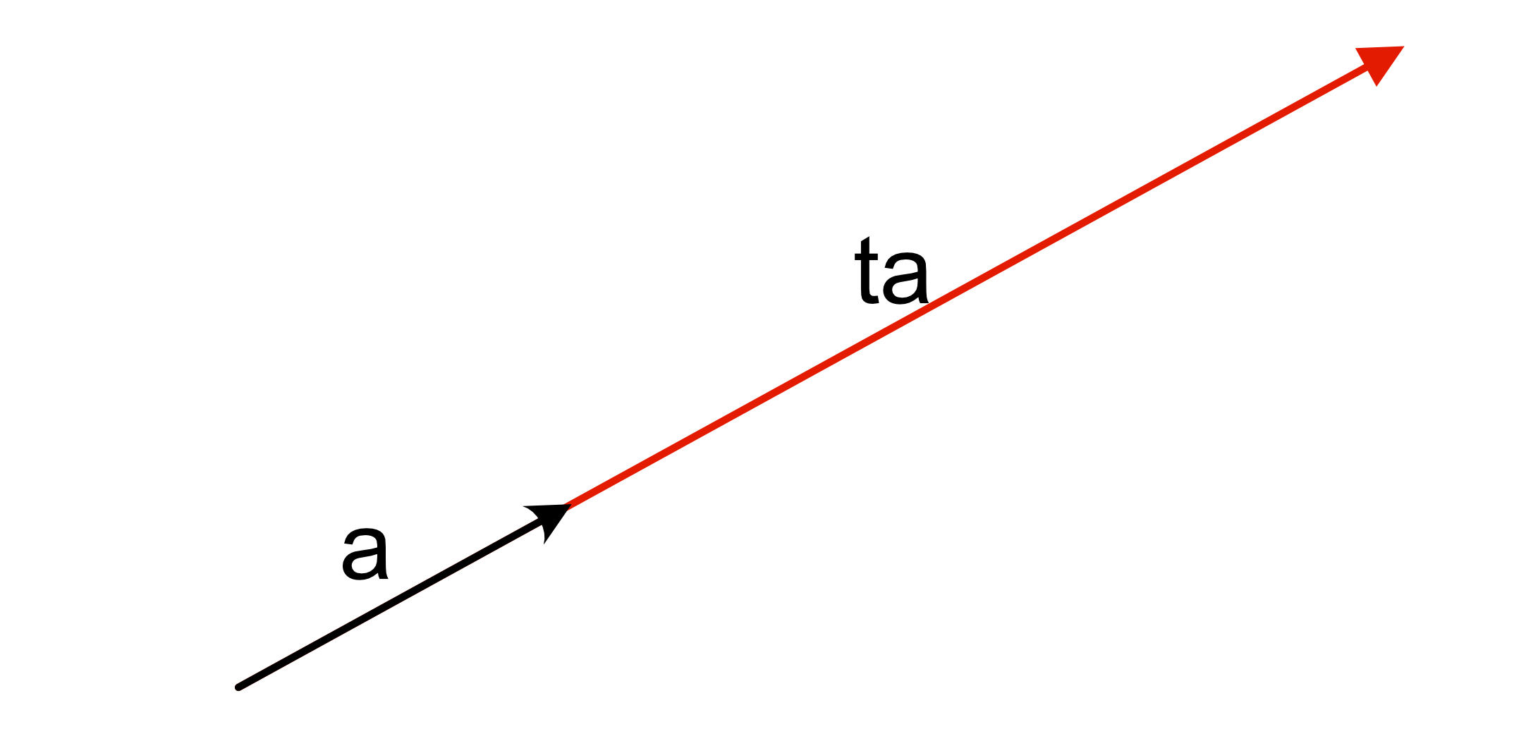
import matplotlib.pyplot as pltDefine a line described by $ \textbf{a} * t$, for example $ \textbf{a} = [1, 0.5]$.
Recall from the reading material that an orthogonal projection is a transformation that maps vectors onto a subspace in such that the distances between original and projected points are minimal.
Example
Define a set of points $X=\begin{bmatrix}|&&|\\x_1&\dots&x_n\\|&&|\end{bmatrix} \in \mathbb{R}^{2\times n}$ (points
in the code) and $\mathbf{a}$ describes a line given by the function $f(x)=0.5x$. The following example will project $X$ onto $\mathbf{a}$:
# Three points
X = np.array([
    [1, 2],
    [2, 1.5],
    [3, 1.2]
]).T

# Show plot
plt.scatter(X[0, :], X[1, :], c="r")

# Make line points (remember Numpy broadcasting)
x = np.linspace(0, 4)
f_x = x * 0.5

# Plot line
# Add grid lines
plt.grid(True)
plt.plot(x, f_x)
plt.xlabel("X coordinates")
plt.ylabel("Y coordinates")
plt.show()
A point $x_i$ is projected onto the vector $\mathbf{a}$ by multiplying $Px_i$ where $P$ is the projection matrix. Projecting all points in $X$ onto the vector $\mathbf{a}$ is therefore $X^{\prime}=PX$.
The projection matrix $P$ is given by:
$$ P = A(A^TA)^{-1}A^T, $$where $A=\mathbf{a}$ (is a column vector).
The code cell below calculates $P$ and projects $X$ onto $\mathbf{a}$:
##1
#The line l written as the design matrix
A = np.array([[1, 0.5]]).T  #  has to be a column vector

##2
## construct projection matrix
P = (A @ np.linalg.inv(A.T @ A)) @ A.T
print("P:\n", P)

#projection the points with matrix multiplication
x_prime = P @ X
print("projected points:\n", x_prime)
P: [[0.8 0.4] [0.4 0.2]] projected points: [[1.6 2.2 2.88] [0.8 1.1 1.44]]
The projection process is visualized below:
# Creating a square figure (makes it easier to visually confirm projection)
plt.figure(figsize=(8, 8))

plt.scatter(X[0, :], X[1, :], label="Original points")  # Old points
plt.scatter(x_prime[0, :], x_prime[1, :], label="Projected points")  # Projected points
plt.plot(x, f_x, label="Line")  # Line
plt.legend()

# Gather old and projected points in a single array
P1 = np.concatenate([X.T[:, :].reshape(1, 3, 2), x_prime.T[:, :].reshape(1, 3, 2)], axis=0)
# Plot projection/error lines
plt.plot(P1[:, 0, 0], P1[:, 0, 1], 'g--')
plt.plot(P1[:, 1, 0], P1[:, 1, 1], 'g--')
plt.plot(P1[:, 2, 0], P1[:, 2, 1], 'g--')
# Add grid lines
plt.grid(True)
# Set axes limits to be the same for equal aspect ratio
plt.xlim(0, 3.5)
plt.ylim(0, 3.5)
plt.xlabel("X coordinates")
plt.ylabel("Y coordinates")
This tutorial is about fitting a straight line (model) to a set of points (matrix $X$). The goal is to find the line that minimizes the error between the actual points and the points predicted by the model.
## 3
# Define the example points
X = np.array([
    [1, 1],
    [2, 2],
    [3, 2]
]).T

plt.grid(True)
plt.scatter(X[0, :], X[1, :])
plt.xlabel("X coordinates")
plt.ylabel("Y coordinates")
# Display the plot
plt.show()
In the previous section, the set of points were projected onto an existing line. In this section, projections are used to perform linear least squares to find model parameters. The model is $f_\mathbf{w}(x) = y = \mathbf{w}_1x + \mathbf{w}_2$, where $x$ is the input and $\mathbf{w}_1$, $\mathbf{w}_2$ are the parameters. The model can be expressed as an inner product $f_\mathbf{w}(x) = y = \begin{bmatrix}x& 1\end{bmatrix}\mathbf{w}$.
With multiple points, a linear set of equations is given by
$$ \begin{bmatrix}x_1 & 1\\\vdots & \vdots \\x_n&1\end{bmatrix} \mathbf{w} = A\mathbf{w} = \mathbf{y} = \begin{bmatrix}y_1\\ \vdots \\y_n\end{bmatrix}. $$Two points are necessary to solve for the model parameters using inverses ($A$ is square). When the set of points $X$ contains more than two points, a linear least squares solution for $\mathbf{w}$ is needed.
A least squares solution implies that there will be some error between $\mathbf{y}$ and the predicted points $\mathbf{\hat{y}}=A\mathbf{w}$. Additionally, $\mathbf{\hat{y}}$ must be in the span of $A$ since it is a linear combination of its column vectors. This is visualized for two dimensions in Figure 2. Observe that $\mathbf{\hat{y}}$ in the figure must be on the line spanned by $A$.
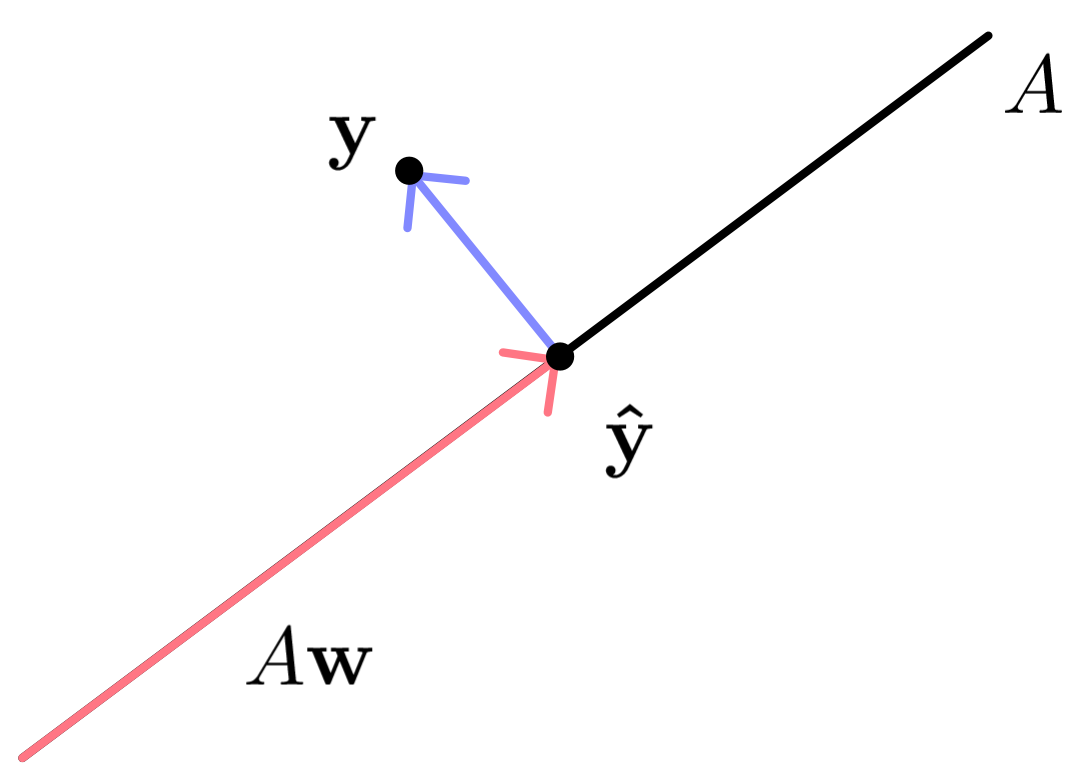
Least squares demonstrations using a two-dimensional design matrix. It visualizes how $\mathbf{\hat{y} }$ is the projection of $\mathbf{y}$ onto $A$ and that $\mathbf{\hat{y} }=A\mathbf{w}$. It also shows the error vector $e$.
Minimizing the error is done by projecting $\mathbb{y}$ onto $A$ as demonstrated for two dimensions in Figure 2. This reveals the relation $\mathbf{\hat{y}} = P\mathbf{y}$ and hence $A\mathbf{w} = P \mathbf{y}=A(A^\top A)^{-1}A^\top \mathbf{y}$.
The final step is solving for $\mathbf{w}$. Since $A$ is multiplied on both sides, isolating $\mathbf{w}$ yields: $$ \mathbf{w} = (A^\top A)^{-1}A^\top \mathbf{y}. $$
Define matrix $A$ with the following columns:
x_vals = X[0, :]
y_vals = X[1, :]

A = np.vstack((x_vals, np.ones(x_vals.shape))).T
print("A\n", A)
A [[1. 1.] [2. 1.] [3. 1.]]
The following cell implements the solution for $\mathbf{w}$ described above:
P = np.linalg.inv(A.T @ A) @ A.T
# Applying the transformation
w = P @ y_vals
print("w:", w)
w: [0.5 0.66666667]
To get the predicted points $\mathbf{\hat{y}}$, $A$ is multiplied onto the parameter vector:
# Calculating the projected y-values
y_hat = A @ w
The w
vector is of the form $(a, b)$ and the line formula is $f(x)=ax+b$. Below, we calculate a number of points on the line for visualization purposes and compare with both the original and projected points:
x = np.linspace(0, 5)  # Create range of values
y = x * w[0] + w[1]  # Calculate f(x)

plt.figure(figsize=(5, 5))

plt.plot(x, y)  # Plot line
plt.scatter(X[0, :], X[1, :])  # Plot original points

plt.scatter(X[0, :], y_hat)  # Plot the points
plt.title('Least squares linear regression 3 points')
plt.xlabel("X coordinates")
plt.ylabel("Y coordinates")
plt.grid(True)
plt.show()
$\mathbf{y}$ and $\mathbf{\hat{y}}$ are both vectors. The projection error is:
$$ e = \|\mathbf{y}-\mathbf{\hat{y}}\| = \sqrt{\sum_{i=1}^n (y_i - \hat{y}_i)^2} = \sqrt{(\mathbf{y}-\mathbf{\hat{y}})(\mathbf{y}-\mathbf{\hat{y}})^\top}. $$# Calculating the error
diff = y_vals - y_hat
e = np.sqrt(diff @ diff.T)
print("e", e)e 0.4082482904638632
To get the mean error, we use
$$ RMS(\mathbf{y}, \mathbf{\hat{y}}) = \sqrt{\frac{1}{n} \sum_{i=1}^n (y_i - \hat{y}_i)^2} = \sqrt{\frac{1}{n}(\mathbf{y}-\mathbf{\hat{y}})(\mathbf{y}-\mathbf{\hat{y}})^\top}. $$diff = y_vals - y_hat
rms = np.sqrt((diff @ diff.T).mean())
print("root mean squared error", rms)root mean squared error 0.4082482904638632