Home
Course Guidelines
About the course Prerequite Material References
Python
Jupyter Notebooks Python overview
Exercises
Before the semester start: Installation and exercise setup Week 1: Introduction to Python and libraries Week 2: Vector representations Week 3: Linear Algebra Week 4: Linear Transformations Week 5: Models and least squares Week 6: Assignment 1 - Gaze Estimation Week 7: Model selection and descriptive statistics Week 8: Filtering Week 9: Classification Week 10: Evaluation Week 11: Dimensionality reduction Week 12: Clustering and refresh on gradients Week 13: Neural Networks Week 14: Convolutional Neural Networks (CNN's)
Tutorials
Week 1: Data analysis, manipulation and plotting Week 2: Linear algebra Week 3: Transformations tutorial Week 4: Projection and Least Squares tutorial Week 7: Cross-validation and descriptive statistics tutorial Week 8: Filtering tutorial Week 11: Gradient Descent / Ascent
In-class Exercises
In-class 1 In-class 2 In-class 10 In-class 3 In-class 4 In-class 8
Explorer

Document

  • Overview
  • 1. Optimization
  • 2. NN architectures
  • 3. Bias variance and regularization

Content

  • Modifying hyperparameters
    • Multilayer Perceptron
      • Task 1 Training basic MLP
      • Task 2 Evaluation
      • Task 3 Training basic MLP modifying hyperparameters
      • Task 4 Comparison
    • Convolutional Neural Network
      • Task 5 CNN architecture
      • Task 6 Training a basic CNN
      • Task 7 Evaluation
      • Task 8 Training a basic CNN modifying hyperparameters
  • Comparing the different model archi…
    • Task 9 Evaluation
    • Task 10 Evaluation
  • Modifying architectures
    • MLP
      • Task 11 Adding a hidden layer
      • Task 12 Compare performance
      • Task 13 Compare architectures
      • Task 14 Compare performance
      • Task 15 Update architecture
  • Convolutional Neural Network
    • Task 16 Adding a convolutional layer
    • Task 17 Compare architectures
    • Task 18 Compare architectures
    • Task 19 Additional improvements

Neural network architectures

This exercise focuses on the classification of the FashionMNIST dataset using two types of neural network architectures: the Multi-Layer Perceptron (MLP) and the Convolutional Neural Network (CNN). The performance of these models will be assessed using the evaluation metrics introduced in earlier exercises.

List of individual tasks
  • Task 1: Training basic MLP
  • Task 2: Evaluation
  • Task 3: Training basic MLP modifying hyperparame…
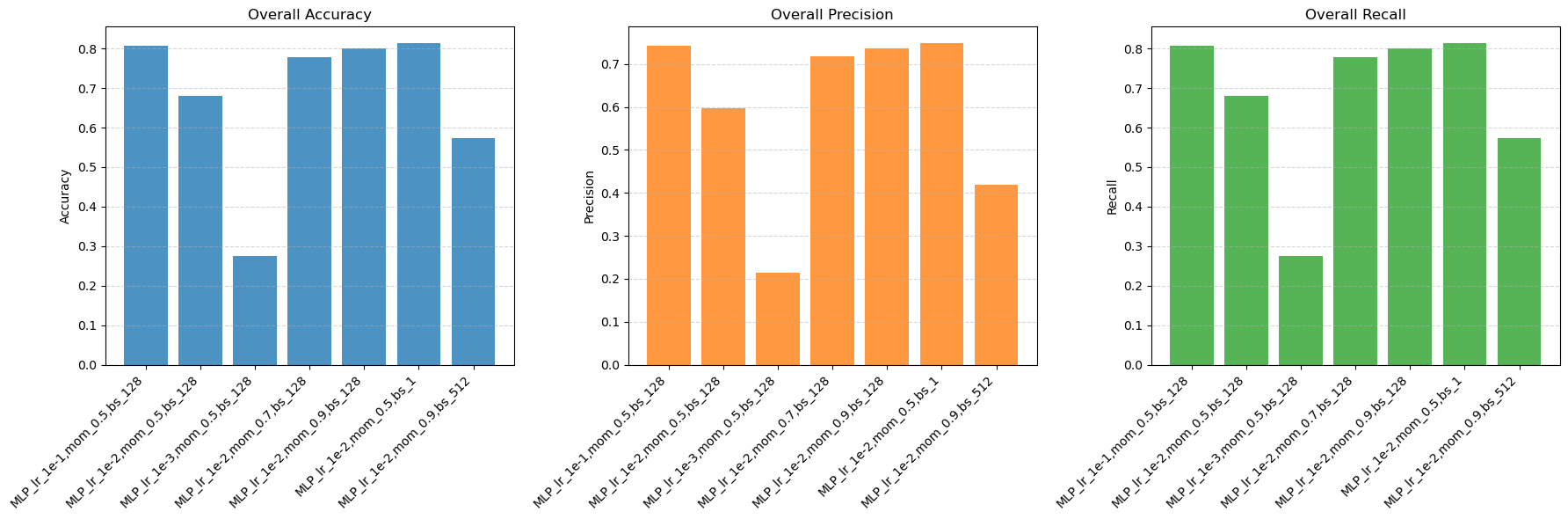
  • Task 4: Comparison
  • Task 5: CNN architecture
  • Task 6: Training a basic CNN
  • Task 7: Evaluation
  • Task 8: Training a basic CNN modifying hyperpara…
  • Task 9: Evaluation
  • Task 10: Evaluation
  • Task 11: Adding a hidden layer
  • Task 12: Compare performance
  • Task 13: Compare architectures
  • Task 14: Compare performance
  • Task 15: Update architecture
  • Task 16: Adding a convolutional layer
  • Task 17: Compare architectures
  • Task 18: Compare architectures
  • Task 19: Additional improvements
Time sink warning

This exercise examines the impact of network architectures and hyperparameters on training and performance. Notice getting optimal results can become a time sink. Make well-argued choices as endless options and combinations are available. Focus on informed decisions given the vast number of options available. Most of the code is provided requiring only modifications to hyperparameter settings and network architecture. This setup allows for focused analysis of outcomes and their connection to theoretical concepts.

Modifying hyperparameters

This part of the exercise introduces and experiments with the hyperparameters of an NN such as the Learning rate and the batch size.

Multilayer Perceptron

The following tasks are about training and modifying an MLP to classify the FashionMNIST dataset. The following functions will be used throughout the exercise:

  • train_pytorch_network : takes an NN class as a parameter. Used for model training and for visualizing the performance of the models throughout the exercise.
  • evaluate_overall_metrics in the cnn_util.py file takes a dictionary containing a key-value pair of a name and a file path to the trained model and a list with the class names. The function returns a plot showing the overall accuracy, precision and recall for the validation data, comparing each model trained.
  • evaluate in the cnn_util.py file takes a dictionary containing a key-value pair of a name and a file path to the trained model and a list with the class names. The function computes a confusion matrix as well as provides plots visualizing Accuracy, Precision and Recall class-wise for the validation data, comparing each model trained.
Task 1: Training basic MLP
  1. Examine the networks.py file and locate the MLPBasic() class. Examine the class to gain an overview of the network architecture.
  2. Run the cell below to train the MLP. The cell will automatically save the trained model in the models/ directory.
from torch import optim from trainers import PyTorchTrainer from networks import * from torchvision import transforms from cnn_util import * from fashionmnist_utils.mnist_reader import load_mnist # uncomment if not first run #from models import * import pandas as pd import numpy as np import matplotlib.pyplot as plt import seaborn as sns import os # Create the 'models' folder os.makedirs("models", exist_ok=True) # Create the 'runs' folder os.makedirs("runs", exist_ok=True) def train_pytorch_network(to_train): transform = transforms.ToTensor() ## conversion from PIL image format to torch tensors. network = to_train trainerNetwork = PyTorchTrainer( nn_module=network, transform=transform, optimizer=optim.SGD(network.parameters(), lr=1e-2, momentum=0.5), batch_size=128 ) print("training the network started") classes = ['t-shirt','trouser','pullover','dress','coat','sandal','shirt','sneaker','bag','ankle boot'] trainerNetwork.train(10) trainerNetwork.plot_metrics(classes) # Evaluate the model logger, predictions = trainerNetwork.evaluate() trainerNetwork.save() print("training and saving the network ended")
from torch import optim
from trainers import PyTorchTrainer
from networks import *
from torchvision import transforms
from cnn_util import *
from fashionmnist_utils.mnist_reader import load_mnist

# uncomment if not first run
#from models import *

import pandas as pd
import numpy as np
import matplotlib.pyplot as plt
import seaborn as sns
import os

# Create the 'models' folder
os.makedirs("models", exist_ok=True)
# Create the 'runs' folder
os.makedirs("runs", exist_ok=True) 


def train_pytorch_network(to_train):

    transform = transforms.ToTensor() ## conversion from PIL image format to torch tensors.

    network = to_train

    trainerNetwork = PyTorchTrainer(
        nn_module=network,
        transform=transform,
        optimizer=optim.SGD(network.parameters(), lr=1e-2, momentum=0.5),
        batch_size=128
    ) 

    print("training the network started")
    classes = ['t-shirt','trouser','pullover','dress','coat','sandal','shirt','sneaker','bag','ankle boot']
    trainerNetwork.train(10)
    trainerNetwork.plot_metrics(classes)


# Evaluate the model
    logger, predictions = trainerNetwork.evaluate()
    trainerNetwork.save()
    print("training and saving the network ended")
train_pytorch_network(MLPBasic())
Task 2: Evaluation
  1. Evaluate the performance of the model during training:
    • Inspect the accuracy, loss and training time. What patterns or trends do you observe in the loss and accuracy graphs throughout training?
# Write your reflections here...

The next task experiments with different hyperparameters. Use the functionevaluate_overall_metrics to visualize and compare the overall performance of the models and use the evaluate function to visualise and compare the performance of the models class-wise. Figure 1 provides an example of the type of plots returned by the functions.

Figure 1:

Example of output from the evaluate_overall_metrics function.

Figure 2:

Example of output from the evaluate function.

Task 3: Training basic MLP modifying hyperparameters
  1. Explore how different hyperparameters influence the training and performance of the model:

    • Modify training variables and train new models:
      • Set the learning rate to 1e-3, and 1e-1.
      • Reset the learning rate to 1e-2 then modify the batch size to 1 and 512.
    • Fill the dictionaries below with the paths of the trained models.
    • Visualize the overall metrics of performance for all models trained using the evaluate_overall_metrics function.
    • Visualize the performance by running the evaluate function.
    Hint

    The cell below is a guide for how to load the models after training. The models are located in the models folder.

MLP_models = {'MLP1...': PyTorchTrainer.load('models/MLPBasic1....pkl'), # replace this with your own model 'MLP2...': PyTorchTrainer.load('models/MLPBasic2....pkl'), # replace this with your own model # Add more... }
MLP_models = {'MLP1...': PyTorchTrainer.load('models/MLPBasic1....pkl'), # replace this with your own model
    'MLP2...': PyTorchTrainer.load('models/MLPBasic2....pkl'), # replace this with your own model
    # Add more...
    }
Task 4: Comparison
  1. Compare the performance of the models:
    • Evaluate the models using accuracy, precision, recall, and heatmaps.
    • Discuss how the changes in hyperparameters, such as learning rate and batch size, influence these performance metrics. Highlight any trends or trade-offs observed, such as improvements in accuracy versus potential declines in precision or recall.
  2. How is the training time affected by the different hyperparameters?
# Write your reflections here...

Convolutional Neural Network

The following tasks investigate a CNN architecture for the same problem.

Task 5: CNN architecture
  1. Locate the CNNBasic model defined in networks.py and explain the architecture.
# Write your explanation here...
Task 6: Training a basic CNN
  1. Run the cell below to train the CNNBasic model.
train_pytorch_network(CNNBasic())
Task 7: Evaluation
  1. Analyze the training figures and describe the key characteristics of the model’s training process.
# Write your reflections here...
Task 8: Training a basic CNN modifying hyperparameters
  1. Experiment with the different hyperparameters affecting the training and performance of the model.
    • Modify the following hyperparameters and train new model:
      • Set the learning rate to 1e-4, and 1e-5.
      • Modify the batch size to 256 and 1024.
    • Fill the dictionary below with the paths of the trained models.
    • Visualize the overall performance by running evaluate_overall_metrics function.
    • Visualize the class-wise performance by running the evaluate function.
CNN_models = {'CNN1...': PyTorchTrainer.load('models/CNNBasic1....pkl'), # replace this with your own model 'CNN2...': PyTorchTrainer.load('models/CNNBasic2....pkl'), # replace this with your own model # Add more... }
CNN_models = {'CNN1...': PyTorchTrainer.load('models/CNNBasic1....pkl'), # replace this with your own model
    'CNN2...': PyTorchTrainer.load('models/CNNBasic2....pkl'), # replace this with your own model
    # Add more...
    }

Comparing the different model architectures

Task 9: Evaluation

In the cell below:

  1. Select the best performing MLP and CNN and update the cell below to store these models in the MLPCNN_models dictionary.
  2. Use the evaluate_overall_metrics function to visualize the overall performance of the models.
  3. Use the evaluate function to visualize the class-wise performance of the models.
MLPCNN_models = {'MLP1...': PyTorchTrainer.load('models/MLPBasic1....pkl'), # replace this with your own model 'CNN1...': PyTorchTrainer.load('models/CNNBasic2....pkl'), # replace this with your own model # Add more... }
MLPCNN_models = {'MLP1...': PyTorchTrainer.load('models/MLPBasic1....pkl'), # replace this with your own model
    'CNN1...': PyTorchTrainer.load('models/CNNBasic2....pkl'), # replace this with your own model
    # Add more...
    }

Evaluate the performance of the different architectures.

Task 10: Evaluation
  1. Training

    • Analyze the figures and explain the key characteristics of the training process for the models.
  2. Metrics

    • Assess the performance of the models by examining the confusion matrices and comparing the MLP and CNN models in terms of accuracy, precision, and recall. Discuss the strengths and weaknesses of each model based on the metrics.
# Write your reflections here...

Modifying architectures

The next part of the exercise is about experimenting with the architecture of an NN such as number of layers, number of perceptrons (nodes) and kernel size.

MLP

The following task will add a hidden layer to the MLP model.

Task 11: Adding a hidden layer
  1. Locate the class MLP_modified in the networks.py file. The MLP_modified class is a copy of the MLPBasic and the following steps are about making changes in the architecture.
  2. Modify the architecture by adding a new hidden layer with 256 nodes, by updating the constructor. Ensure that the number of input and output features match between the layers.
  3. Update the forward function to ensure this new hidden layer is used in the predictions.
  4. Train the model by running the cell below.
train_pytorch_network(MLP_modified())
Task 12: Compare performance
  1. Examine the training figures to identify and explain the characteristics of the model’s training process.
# Write your reflections here ...

Evaluate the modified MLP against the MLPBasic()

Task 13: Compare architectures

In the cell below:

  1. Identify the best-performing MLP and MLPModified models based on the evaluation metrics. Update the cell below to store these selected models in the modelsMLPModified dictionary.
  2. Use the evaluate_overall_metrics function to visualize the overall performance of the models.
  3. Use the evaluate function to visualize the class-wise performance of the models.
MLPModified_model = {'MLP1...': PyTorchTrainer.load('models/MLP1....pkl'), # replace this with your own model 'MLP_mod1...': PyTorchTrainer.load('models/MLP_mod1....pkl'), # replace this with your own model 'MLP_mod2...': PyTorchTrainer.load('models/MLP_mod2....pkl'), # replace this with your own model # Add more... }
MLPModified_model = {'MLP1...': PyTorchTrainer.load('models/MLP1....pkl'), # replace this with your own model
    'MLP_mod1...': PyTorchTrainer.load('models/MLP_mod1....pkl'), # replace this with your own model
    'MLP_mod2...': PyTorchTrainer.load('models/MLP_mod2....pkl'), # replace this with your own model
    # Add more...
    }
Task 14: Compare performance
  1. Evaluate the performance of the models by analyzing the confusion matrices. Compare the MLP and CNN models in terms of key metrics such as accuracy, precision, and recall, and provide a detailed explanation of their relative strengths and weaknesses based on these metrics
# Write your reflections here...
Task 15: Update architecture
  1. Change the number of hidden nodes to 512 (adjust the other layers accordingly).
  2. Rerun the cell above to train the new model.
  3. Include the new model in the dictionary.
  4. Evaluate the model and compare it with the others as in Task 13.

Convolutional Neural Network

The following task will involve modifying the architechture of the CNN.

Hint
  • Recall that the kernel size influences the size of the output image. Specifically, for kernel size $k$, the output has dimensions $w-(k-1) \times h-(k-1)$ where $w$ is the width and $h$ is the height of an image. Adding a convolutional layer is consequently a bit more tricky than a linear layer because the dimensions between the layers need to match. You will likely need to debug the model a few times to get it right, therefor we encourage you to carefully examine the structure of the network before modifying it.
  • Convolutional layers MAY be accompanied with a max pooling layer, but remember to use an activation function.
  • The max_pool2d operation in theforward function halves the image resolution.
Task 16: Adding a convolutional layer
  1. Locate the class CNN_modified() in the networks.py file.
  2. Examine the class to gain an overview of the network architecture. Note that it is a copy of the CNNBasic() class.
  3. Add a new Conv2d layer to the CNN_modified class by decreasing the kernel size of the existing first layer and add the new layer as the second layer.
Hint

Use tensor.size to get the size of any tensor.

  1. Update the forward method to ensure this new hidden layer is used in the predictions.
  2. Train the model by running the cell below.
train_pytorch_network(CNN_modified())
Task 17: Compare architectures
  1. Fill in the dictionary below with the best performing CNNBasic() model and the CNNModified() .
  2. Visualize the overall performance by running evaluate_overall_metrics function.
  3. Visualize the class-wise performance by running the evaluate function.
CNNModified_model = {'CNN1...': PyTorchTrainer.load('models/CNN1....pkl'), # replace this with your own model 'CNN_mod1...': PyTorchTrainer.load('models/CNN_mod1....pkl'), # replace this with your own model 'CNN_mod2...': PyTorchTrainer.load('models/CNN_mod2....pkl'), # replace this with your own model # Add more... }
CNNModified_model = {'CNN1...': PyTorchTrainer.load('models/CNN1....pkl'), # replace this with your own model
    'CNN_mod1...': PyTorchTrainer.load('models/CNN_mod1....pkl'), # replace this with your own model
    'CNN_mod2...': PyTorchTrainer.load('models/CNN_mod2....pkl'), # replace this with your own model
    # Add more...
    }
Task 18: Compare architectures

Evaluate the modified CNN against the CNNBasic() following the steps:

  1. During training:

    • Include the trained CNNBasic() and the CNNModified() in the graphs (leave out the rest).
    • What patterns or trends do you observe in the loss and accuracy graphs and training time throughout training?
  2. Update the dictionary below with the trained models and execute the cell. Compare the performance of the models, providing an analysis and explanation of the observed differences.

  3. Change the kernel size and the number of kernels to achieve the best performing model, while avoiding overfitting. Run the cell above to train the new model. Include the new model in the dictionary, evaluate the model and compare it with the others.

# Write your reflections here...

This exercise has briefly introduced some modifications that can improve the performance of a model. While this was just a brief introduction many more alterations can be performed. However, as noted, this easily becomes a time sink. The next task is optional and continues the introduction of possible alterations.

Task 19: Additional improvements (optional)

Change the activation functions, the number of hidden layers, and the training setup to achieve the best performing model. Notice, that a huge amount of time can be spent on fiddling with the models.