PCA for shape generation

Data

The dataset used for the assigment consist of 120 landmarks (2D points) of faces (data space). A face consists of 73 (x,y)-coordinate pairs, i.e. 146 featues in total.

## Importing libraries
import matplotlib.pyplot as plt
import numpy as np
import scipy
from pca_utils import *
import os
from glob import glob

path = './db/'
shapes, _ = face_shape_data(path)

plot_many_faces(shapes[:6],"Original face shapes");

PCA implementation

The following tasks are about using the implementation of PCA from the in-class exercise on the face shape dataset.

# 1
def get_principal_components(X):
    """Calculates principle components for X.

    Args:
        X: The dataset. An NxD array were N are the number of samples and D are
        the number of features.

    Returns:
        Tuple (components, eigenvalues, mu) where components is a DxD matrix of
        principle components, eigenvalues is a D-element vector of
        corresponding eigenvalues, and mu is a D-element array containing the mean
        vector.
    """
    # Copy your PCA implementation to here.


# 2, 3 and 4
# Get the principal components for the dataset and transform the faces to feature space.
comp, val, mu = get_principal_components(shapes)

# write code for finding the cumulative proportional variance here

# selecting 5 components 
n_components = 5


# 5
def transform_to_latent_space(X, principle_components, mu):
    """Transforms X to an k-dimensional space where k is the number of
    principle_components.

    Args:
        X: The dataset. An NxD array were N are the number of samples and D are
        the number of features.
        principle_components: An Dxk matrix containing the principle
        components.
        mu: A D-element array containing the mean vector.

    Returns:
        A Nxk array describing the transformed data.
    """
    #return ...

    
# 6  
def transform_from_latent_space(v, principle_components, mu):
    """Reverses the dimensionality reduction of v, a Nxk matrix where
    k is the number of principle components. The result is a NxM matrix.

    Args:
        v: The transformed dataset with size Nxk.
        principle_components: An Dxk matrix containing the principle
        components.
        mu: A Mx1 matrix containing the mean vector.

    Returns:
        An NxD array reconstruction of the original feature vectors X.
    """
    #return ...

    
# 7     
used = comp[:, :n_components]

# transforming and reconstructing the 6 first faces in the dataset
plot_many_faces(shapes[:6],"Original face shapes")
transformed = transform_to_latent_space(shapes[:6], used, mu)
restored = transform_from_latent_space(transformed, used, mu)
plot_many_faces(restored,"Restored faces using 5 principal components")

2 first principal components have a cumulative proportional variance of: [0.37823316 0.66546276] 

Using PCA for shape generation

The principal components can be used to generate new samples $\mathbf{x}$ in data space by transforming a point in latent space according to $$ \mathbf{x} = \Phi_{k} a + \mu $$ where $\Phi_{k}$ is the matrix of k eigenvectors, $\mathbf{a}\in\mathbb{R}^{k}$ is a vector in latent space, and $\mu\in\mathbb{R}^{D}$ is the mean vector of the original data features in the data space.

The variance of the data in a given direction can be used to constrain the values of the elements of the vector $\mathbf{a}$ in latent space, assuming that the data follows a (multivariate) normal distribution. In a multivariate normal distribution each direction $v_i$ is also normally distributed. Each element $a_i$ can be constrained to be within the observed variance in direction $v_i$. The variance $\sigma_i^2$ in the direction of $v_i$ is given by the eigenvalue $\lambda_i$, so the standard deviation is $\sigma_i = \sqrt{\lambda_i}$.

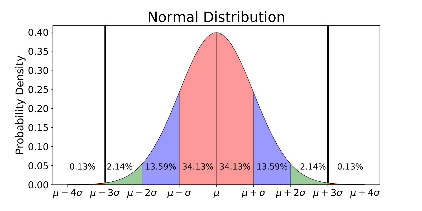
In a 1D normal distribution (with mean $\mu$ and standard deviation $\sigma$), the area under the Gaussian curve between $\pm 3\sigma$ contains $99.7\%$ of the data (see Figure 1 ). Thus, constraining each element $a_i$ to the interval $[-3\sigma_i, 3\sigma_i]$ will cover $99.7\%$ of the variance in the direction of $v_i$.

a = np.array([0,0,0,0,0])

# Write your implementation here.

# Write your reflections here

Investigating principal components

The following tasks are about investigating properties of principal components.

std_1 = np.sqrt(val[0]) # std/eigvalue for the first PC
np.linspace(-3*std_1, 3*std_1, num=5)

# Write your solution here

plot_many_faces(gen_shapes,"Generated face shapes by varying the first coordinate in latent space")

# Write your reflections here

Interpolating between shapes

The following example shows how to interpolate two vectors.

# #Template for doing interpolation between two (2D)- points 
d = np.linspace(np.array([1, 2]), np.array([3, 5]), num=5)
plt.scatter(d[:, 0], d[:, 1])

# write the implementation for "Interpolation between two faces" here

# Write reflections here.

Last section - optional

This final section includes three tasks that offer valuable insights into the application of PCA, however completing this section is optional.

def get_principal_components_correlation(X):
    """Calculates principal components using the correlation matrix for X.

    Args:
        X: The dataset. An NxD array where N are the number of samples and D are
        the number of features.

    Returns:
        Tuple (components, eigenvalues, mu) where components is a DxD matrix of
        principal components, eigenvalues is a D-element vector of
        corresponding eigenvalues, and mu is a D-element array containing the mean
        vector.
    """
    # Standardize the data
    
    # Compute the correlation matrix
    
    # Sort the eigenvalues and eigenvectors in descending order
    
    return ....

# Use the function on the shapes data
eigenvectors_corr, eigenvalues_corr, mu_corr = get_principal_components_correlation(shapes)

# Optionally, plot the eigenvalues to see their distribution
plt.figure(figsize=(8, 6))
plt.plot(range(1, len(eigenvalues_corr) + 1), eigenvalues_corr, 'o-', linewidth=2)
plt.title('Eigenvalues of the Correlation Matrix')
plt.xlabel('Principal Component')
plt.ylabel('Eigenvalue')
plt.grid(True)
plt.show()

variance_explained = eigenvalues_corr / np.sum(eigenvalues_corr)
cumulative_variance_explained = np.cumsum(variance_explained)

# Plot cumulative variance explained
plt.figure(figsize=(8, 6))
plt.plot(range(1, len(cumulative_variance_explained) + 1),
         cumulative_variance_explained, 'o-', linewidth=2)
plt.title('Cumulative Variance Explained by Principal Components')
plt.xlabel('Number of Principal Components')
plt.ylabel('Cumulative Variance Explained')
plt.axhline(y=0.95, color='r', linestyle='--')  # Line to indicate 90% variance
plt.grid(True)
plt.show()

# Write implementation here

Describe the different scatter plots of component combinations

# Write implementation and reflections here