Home
Course Guidelines
About the course Prerequite Material References
Python
Jupyter Notebooks Python overview
Exercises
Before the semester start: Installation and exercise setup Week 1: Introduction to Python and libraries Week 2: Vector representations Week 3: Linear Algebra Week 4: Linear Transformations Week 5: Models and least squares Week 6: Assignment 1 - Gaze Estimation Week 7: Model selection and descriptive statistics Week 8: Filtering Week 9: Classification Week 10: Evaluation Week 11: Dimensionality reduction Week 12: Clustering and refresh on gradients Week 13: Neural Networks Week 14: Convolutional Neural Networks (CNN's)
Tutorials
Week 1: Data analysis, manipulation and plotting Week 2: Linear algebra Week 3: Transformations tutorial Week 4: Projection and Least Squares tutorial Week 7: Cross-validation and descriptive statistics tutorial Week 8: Filtering tutorial Week 11: Gradient Descent / Ascent
In-class Exercises
In-class 1 In-class 2 In-class 10 In-class 3 In-class 4 In-class 8
Explorer

Document

  • Overview
  • 1. Classification and decision boundaries
  • 2. Introduction to Logistic Regression
  • 3. Histogram of Oriented Gradients (HOG)

Content

  • Experimenting with model parameters…
    • Task 1 Implementing the sigmoid function
    • Task 2 The prediction function
    • Task 3 Evaluation
    • Task 4 Increasing input dimensions
    • Task 5 2D Predictions
    • Task 6 Reflection and plotting 2D
    • Task 7 Plotting in 3D

Introduction to Logistic Regression

In this exercise, you will explore the characteristics of the logistic classifier.

List of individual tasks
  • Task 1: Implementing the sigmoid function
  • Task 2: The prediction function
  • Task 3: Evaluation
  • Task 4: Increasing input dimensions
  • Task 5: 2D Predictions
  • Task 6: Reflection and plotting 2D
  • Task 7: Plotting in 3D

The figure below shows a schematic of a multivariate logistic regression classifier.

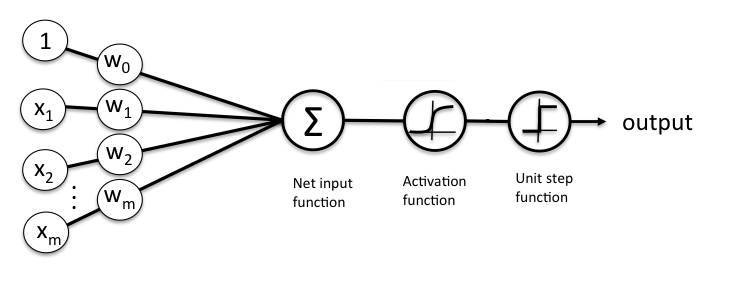
A Logistic regression classifier consists of 3 distinct parts:

  1. A multivariate linear function : $z = \mathbf{w}^\top\mathbf{x} = \sum_i w_i*x_i +w_0$ , where $\mathbf{w}$ are the model parameters (including the bias term $w_0$) and $\mathbf{x}$ the homogeneous coordinates of the input

  2. The sigmoid activation function $\sigma(z)=\frac{1}{1+\text{e}^{(-z)}}$

  3. A binary step function (thresholding) at $\sigma(z)>0.5$.

The libraries used are imported in the next cell.

import numpy as np import matplotlib.pyplot as plt
import numpy as np
import matplotlib.pyplot as plt

Experimenting with model parameters of the logistic (regression) classifier

Task 1: Implementing the sigmoid function

In the following task you will implement steps 1 and 2 from above and visualize the output $\sigma(z)$ along with the decision boundary obtained in step 3.

In the cell below:

  1. Implement the function linear_sigmoid , that calculates the variable $z$ as the linear combination of the input features $x$, the weights $w$, the bias $w_0$ and then returns the output of the sigmoid activation function applied to $z$.
  2. Calculate the decision boundary for the logistic regression classifier where $\sigma(z) = 0.5$.
  3. Run the cell below to plot the function values of linear_sigmoid using the values of xs as input, along with the calculated decision boundary.
  4. Modify the model parameters w ($z = \mathbf{w}^\top\mathbf{x} = \sum_i w_i*x_i +w_0$) and observe their effect on the shape of the sigmoid function. What happens to the function when $w_i$:
    • is small? (does it look similar to another function?)
    • is large?
    • is zero?
  5. How does a change of the bias $w_0$ affect the output of linear_sigmoid ?
  6. Determine the x-values of the decision boundary (x-value where $\sigma(x)=0.5$ ) for the logistic regression-classifier.
Hint

z must be zero in:

$$ \sigma(z)=\frac{1}{1+\text{e}^{(-z)}} $$

for $\sigma(z)=0.5$, hence solve $w_0 + w x = 0$

def linear_sigmoid(x,b,w) : # sigmoid function """ :param x: 1D array of the (single) input-feature values. :param b: The bias parameter of the model. :param W: The weight parameter of the model. :return (float): output values of the sigmoid function. """ ... xs = np.linspace(-100,100,1000) ### linspace of "input features" params = [3.0,0.15] ### parameters of the model # Calc decision boundary here Decision_boundary = ... # write your solution here ### plotting #### plt.figure(figsize=(8,6)) plt.plot(xs, linear_sigmoid(xs,params[0],params[1]),label = r"$\sigma(x)$ = 1/(1 + exp(-(%.2f + %.2fx))"%(params[0],params[1])) plt.plot([Decision_boundary,Decision_boundary],[0,1],'--C3',label = 'decision boundary') plt.title(r"Sigmoid $\sigma(x)$", fontsize=20) plt.legend() plt.show()
def linear_sigmoid(x,b,w) :  # sigmoid function
    """
    :param x: 1D array of the (single) input-feature values.
    :param b: The bias parameter of the model.
    :param W: The weight parameter of the model.
    
    :return (float): output values of the sigmoid function. 
    """
    ...

xs = np.linspace(-100,100,1000) ### linspace of "input features"
params = [3.0,0.15] ### parameters of the model

# Calc decision boundary here
Decision_boundary = ... # write your solution here

### plotting ####
plt.figure(figsize=(8,6))
plt.plot(xs, linear_sigmoid(xs,params[0],params[1]),label = r"$\sigma(x)$ = 1/(1 + exp(-(%.2f + %.2fx))"%(params[0],params[1]))
plt.plot([Decision_boundary,Decision_boundary],[0,1],'--C3',label = 'decision boundary')
plt.title(r"Sigmoid $\sigma(x)$", fontsize=20)
plt.legend()
plt.show()

The cell below generates two classes (class1 and class2 ) of data, drawn from normal distributions (with a different mean and variance)

### 2 classes of randomly generated data x1= np.random.normal(-50,20,200) y1 = np.zeros_like(x1) x2= np.random.normal(50,30,200) y2 = np.ones_like(x2)
### 2 classes of randomly generated data

x1= np.random.normal(-50,20,200)
y1 = np.zeros_like(x1)
x2= np.random.normal(50,30,200)
y2 = np.ones_like(x2)

x1 and x2 are the variables for the input features of class1 and class2 , respectively. Likewise, y1 and y2 are the targets of class1 and class2 , respectively.

The following cell visualizes the data of the classes together with the sigmoid values and the decision boundary.

plt.figure(figsize=(8,6)) plt.plot(xs, linear_sigmoid(xs,params[0],params[1]),label = r"$\sigma(x)$ = 1/(1 + exp(-(%.2f + %.2fx))"%(params[0],params[1])) plt.plot(x1, y1+np.random.normal(0,0.01,200),'p',label ='class1') plt.plot(x2, y2+np.random.normal(-0,0.01,200),'o',label = 'class2') plt.plot([-params[0]/params[1],-params[0]/params[1]],[0,1],'--C3',label = 'decision boundary') plt.title(r"Logistic regression and target data", fontsize=20) plt.legend() plt.show()
plt.figure(figsize=(8,6))
plt.plot(xs, linear_sigmoid(xs,params[0],params[1]),label = r"$\sigma(x)$ = 1/(1 + exp(-(%.2f + %.2fx))"%(params[0],params[1]))
plt.plot(x1, y1+np.random.normal(0,0.01,200),'p',label ='class1')
plt.plot(x2, y2+np.random.normal(-0,0.01,200),'o',label = 'class2')
plt.plot([-params[0]/params[1],-params[0]/params[1]],[0,1],'--C3',label = 'decision boundary')

plt.title(r"Logistic regression and target data", fontsize=20)
plt.legend()
plt.show()
Task 2: The prediction function
  1. In the cell below implement the function predict using the linear_sigmoid function and binary thresholding to predict the class given input-features and model parameters.
def predict(x,w): """ :param x: 1D array of the (single) input-feature values. :param w: The list of the model parameters, [bias, weight]. :return: Boolean array same size as x, where a True values signifies class2, and False signifies class1 """ ...
def predict(x,w):
    """
    :param x: 1D array of the (single) input-feature values.
    :param w: The list of the model parameters, [bias, weight]. 
    
    :return: Boolean array same size as x, where a True values signifies class2, and False signifies class1
    """
    ...

The cell below visualizes the predictions.

x_all = np.concatenate([x1,x2]) y_all = np.concatenate([y1+np.random.normal(0,0.01,200),y2+np.random.normal(-0,0.01,200)]) y_bool = predict(x_all,params) plt.figure(figsize=(8,6)) plt.plot(x_all[~y_bool], y_all[~y_bool],'p',color='orange',label ='Predicted class1') plt.plot(x_all[y_bool], y_all[y_bool],'go',label = 'Predicted class2') plt.plot(xs, linear_sigmoid(xs,params[0],params[1]),'b',label = r"$\sigma(x)$ = 1/(1 + exp(-(%.2f + %.2fx))"%(params[0],params[1])) plt.plot([-params[0]/params[1],-params[0]/params[1]],[-0.04,1.04],'--C3',label = 'decision boundary') plt.title(r"Logistic regression prediction", fontsize=20) plt.legend() plt.show()
x_all = np.concatenate([x1,x2])
y_all = np.concatenate([y1+np.random.normal(0,0.01,200),y2+np.random.normal(-0,0.01,200)])
y_bool = predict(x_all,params)
plt.figure(figsize=(8,6))
plt.plot(x_all[~y_bool], y_all[~y_bool],'p',color='orange',label ='Predicted class1')
plt.plot(x_all[y_bool], y_all[y_bool],'go',label = 'Predicted class2')
plt.plot(xs, linear_sigmoid(xs,params[0],params[1]),'b',label = r"$\sigma(x)$ = 1/(1 + exp(-(%.2f + %.2fx))"%(params[0],params[1]))
plt.plot([-params[0]/params[1],-params[0]/params[1]],[-0.04,1.04],'--C3',label = 'decision boundary')
plt.title(r"Logistic regression prediction", fontsize=20)
plt.legend()
plt.show()
Task 3: Evaluation
  1. Visually assess which model parameters w best seperate the two classes?
  2. Determine the accuracy (fraction of correct predictions) of the classifier.
Tip

You can use the accuracy function from the previous exercise.

# Code you solution here
Accuracy of the logistic regression classifier is: 0.963
Task 4: Increasing input dimensions

In this task the logistic regression function is modified to take 2 features as input (x,y).

  1. Complete the sigmoid2D function such that it can take a vector of two 1D-arrays as input.
  2. Run the cell below to visualize a 3D-plot of the 2-variable sigmoid function and the decision boundary plane
  3. The decision boundary is defined by the plane where $z\in[0,1]$ and x,y such that $ b + w_1*x+w_2*y = 0 $ . Why is this?
  4. How does changing the individual model parameters $w_1$ and $w_2$ affect the orientation and slope of the decision boundary plane in the 3D plot?
  5. What happens to the decision boundary if $w_1$ or $w_2$ is set to zero?
def sigmoid2D(X,params) : # sigmoid function """ :param X: tuple of input features (x,y). :param parametes: List of the model parameters. :return: output values of the sigmoid function. """ # Write solutions here ... #### Plotting x = np.linspace(-50, 50, 1000) y = np.linspace(-50, 50, 1000) X, Y = np.meshgrid(x, y) params3 = [0.07,0.037,0.085] Z = sigmoid2D((X, Y),params3) fig = plt.figure(figsize=(15,7)) # ----- First subplot: 3D sigmoid function ----- ax1 = fig.add_subplot(1, 2, 1, projection='3d') # 1 row, 2 columns, first plot # Decision boundary plane calculation y_decision_boundary = -(params3[0]/params3[2]) - (params3[1]/params3[2]) * x # Create mesh for decision boundary plane in 3D space Y_decision, Z_decision = np.meshgrid(y_decision_boundary, np.linspace(0, 1, 1000)) # z from 0 to 1 for probabilities X_decision = np.tile(x, (len(Y_decision), 1)) # x values remain constant for the plane # Plot the decision boundary as a wireframe to make it clearly visible boundary_surface = ax1.plot_wireframe(X_decision, Y_decision, Z_decision, color='black', alpha=0.6, label='Decision Boundary') sigmoid_surface = ax1.plot_surface(X, Y, Z, color='green', alpha=0.3) # making it more transparent ax1.set_title(r"Sigmoid : $\sigma(x,y)$ = 1/(1 + exp(-(%.2f + %.2fx + %.2fy))"%(params3[0],params3[1],params3[2]), fontsize=20) ax1.set_xlabel('X') ax1.set_ylabel('Y') ax1.set_zlabel('Z (Probability)') ax1.view_init(elev=15., azim=2) # ----- Second subplot: 2D projection of the decision boundary ----- ax2 = fig.add_subplot(1, 2, 2) # 1 row, 2 columns, second plot # Plot the decision boundary line ax2.plot(x, y_decision_boundary, color='black',linewidth=3, label='Decision Boundary') ax2.fill_between(x, y_decision_boundary, y[0], color='blue', alpha=0.3, label = 'class 1') # Optional: fill area under the line ax2.fill_between(x, y_decision_boundary, y[-1], color='red', alpha=0.3, label = 'class 2') # Optional: fill area under the line ax2.set_xlabel('X') ax2.set_ylabel('Y') ax2.set_title('Decision Boundary in XY plane', fontsize=14) ax2.legend() plt.tight_layout() plt.show()
def sigmoid2D(X,params) :  # sigmoid function
    """
    :param X: tuple of input features (x,y).
    :param parametes: List of the model parameters.
    :return: output values of the sigmoid function. 
    """
    # Write solutions here
    ...

#### Plotting
x = np.linspace(-50, 50, 1000)
y = np.linspace(-50, 50, 1000)
X, Y = np.meshgrid(x, y)
params3 = [0.07,0.037,0.085]
Z = sigmoid2D((X, Y),params3)

fig = plt.figure(figsize=(15,7))

# ----- First subplot: 3D sigmoid function -----
ax1 = fig.add_subplot(1, 2, 1, projection='3d')  # 1 row, 2 columns, first plot

# Decision boundary plane calculation
y_decision_boundary = -(params3[0]/params3[2]) - (params3[1]/params3[2]) * x

# Create mesh for decision boundary plane in 3D space
Y_decision, Z_decision = np.meshgrid(y_decision_boundary, np.linspace(0, 1, 1000))  # z from 0 to 1 for probabilities
X_decision = np.tile(x, (len(Y_decision), 1))  # x values remain constant for the plane

# Plot the decision boundary as a wireframe to make it clearly visible
boundary_surface = ax1.plot_wireframe(X_decision, Y_decision, Z_decision, color='black', alpha=0.6, label='Decision Boundary')
sigmoid_surface = ax1.plot_surface(X, Y, Z, color='green', alpha=0.3)  # making it more transparent

ax1.set_title(r"Sigmoid : $\sigma(x,y)$ = 1/(1 + exp(-(%.2f + %.2fx + %.2fy))"%(params3[0],params3[1],params3[2]), fontsize=20)
ax1.set_xlabel('X')
ax1.set_ylabel('Y')
ax1.set_zlabel('Z (Probability)')
ax1.view_init(elev=15., azim=2)

# ----- Second subplot: 2D projection of the decision boundary -----
ax2 = fig.add_subplot(1, 2, 2)  # 1 row, 2 columns, second plot

# Plot the decision boundary line
ax2.plot(x, y_decision_boundary, color='black',linewidth=3, label='Decision Boundary')
ax2.fill_between(x, y_decision_boundary, y[0], color='blue', alpha=0.3, label = 'class 1')  # Optional: fill area under the line
ax2.fill_between(x, y_decision_boundary, y[-1], color='red', alpha=0.3, label = 'class 2')  # Optional: fill area under the line

ax2.set_xlabel('X')
ax2.set_ylabel('Y')
ax2.set_title('Decision Boundary in XY plane', fontsize=14)
ax2.legend()

plt.tight_layout() 
plt.show()
# write your reflections here

Identically to above, we generate 2 classes (class1 and class2 ), but this time with two input features.

S = 100*np.eye(2) p1,q1 = np.random.multivariate_normal([20,8], S, 200).T p2,q2 = np.random.multivariate_normal([-10,-13], S, 200).T z1 = np.ones_like(q1)+np.random.normal(0,0.01,200) z2 = np.zeros_like(q2)+np.random.normal(0,0.01,200)
S = 100*np.eye(2)
p1,q1 = np.random.multivariate_normal([20,8], S, 200).T
p2,q2 = np.random.multivariate_normal([-10,-13], S, 200).T

z1 = np.ones_like(q1)+np.random.normal(0,0.01,200)
z2 = np.zeros_like(q2)+np.random.normal(0,0.01,200)
Task 5: 2D Predictions
  1. Implement predict2D , that predicts the class (binary) of a 2D data input.
  2. Use predict2D to determine the accuracy of the logistic classifier.
  3. Manually choose parameters that result in an accuracy above $80\%$
def predict2D(X,params): """ :param x: tuple of 1D arrays of the input-feature values. :param params: The list of the model parameters, [bias, weight1, weight2]. :return: Boolean array same size as x, where a True values signifies class2, and False signifies class1 """ ... # Code you solution here
def predict2D(X,params):
    """
    :param x: tuple of 1D arrays of the input-feature values.
    :param params: The list of the model parameters, [bias, weight1, weight2]. 
    
    :return: Boolean array same size as x, where a True values signifies class2, and False signifies class1
    """
    ...

# Code you solution here
Accuracy of the logistic regression classifier is: 0.037
Task 6: Reflection and plotting 2D
  1. Update the params3 list with the best model parameters from task 3.

Run the cell below to:

  • Plot the generated data together with the 2D input logistic function and decision boundary.
  • Make a 2D projection plot in the XY plane of the decision boundary and the data points. Plot class 1 as blue and class 2 as red.
  1. Consider the last exercise on decision boundaries: are there any similarities between the linear descision boundary and the current 2D projection plot?
# Fill the empty list below with the best model parameters from task 3 params3 = [] x = np.linspace(-50, 50, 1000) y = np.linspace(-50, 50, 1000) X, Y = np.meshgrid(x, y) Z = sigmoid2D((X, Y), params3) # Decision boundary plane calculation y_decision_boundary = -(params3[0] / params3[2]) - (params3[1] / params3[2]) * x # Separate plot for the second subplot fig, ax2 = plt.subplots(figsize=(10, 7)) # Plot the decision boundary line ax2.plot(x, y_decision_boundary, color='black', linewidth=3, label='Decision Boundary') ax2.plot(p1, q1, 'p', color='blue', label='class 1') ax2.plot(p2, q2, 'o', color='red', label='class 2') ax2.fill_between(x, y_decision_boundary, y[0], color='red', alpha=0.3, label='class 2 predictions') ax2.fill_between(x, y_decision_boundary, y[-1], color='blue', alpha=0.3, label='class 1 predictions') ax2.set_xlabel('X') ax2.set_ylabel('Y') ax2.set_title('Decision Boundary in XY plane', fontsize=14) ax2.legend() plt.show()
# Fill the empty list below with the best model parameters from task 3
params3 = []

x = np.linspace(-50, 50, 1000)
y = np.linspace(-50, 50, 1000)
X, Y = np.meshgrid(x, y)
Z = sigmoid2D((X, Y), params3)


# Decision boundary plane calculation
y_decision_boundary = -(params3[0] / params3[2]) - (params3[1] / params3[2]) * x


# Separate plot for the second subplot
fig, ax2 = plt.subplots(figsize=(10, 7))

# Plot the decision boundary line
ax2.plot(x, y_decision_boundary, color='black', linewidth=3, label='Decision Boundary')
ax2.plot(p1, q1, 'p', color='blue', label='class 1')
ax2.plot(p2, q2, 'o', color='red', label='class 2')
ax2.fill_between(x, y_decision_boundary, y[0], color='red', alpha=0.3, label='class 2 predictions')
ax2.fill_between(x, y_decision_boundary, y[-1], color='blue', alpha=0.3, label='class 1 predictions')

ax2.set_xlabel('X')
ax2.set_ylabel('Y')
ax2.set_title('Decision Boundary in XY plane', fontsize=14)
ax2.legend()

plt.show()
Task 7: Plotting in 3D
  1. Consider the 3D plot below. Update the params3 list with the best model parameters from task 3.

Run the cell below, then compare your plots to the 2D plot:

  1. Which plot do you prefer. Argue for your choice.
# Fill the empty list below with the best model parameters from task 3 params3 = [] # Plotting data point along with the sigmoid x = np.linspace(-50, 50, 1000) y = np.linspace(-50, 50, 1000) X, Y = np.meshgrid(x, y) Z = sigmoid2D((X, Y),params3) fig = plt.figure(figsize=(15,7)) # ----- First subplot: 3D sigmoid function ----- ax1 = fig.add_subplot(1, 1, 1, projection='3d') # 1 row, 2 columns, first plot # Decision boundary plane calculation y_decision_boundary = -(params3[0]/params3[2]) - (params3[1]/params3[2]) * x # Create mesh for decision boundary plane in 3D space Y_decision, Z_decision = np.meshgrid(y_decision_boundary, np.linspace(0, 1, 1000)) # z from 0 to 1 for probabilities X_decision = np.tile(x, (len(Y_decision), 1)) # x values remain constant for the plane # Plot the decision boundary as a wireframe to make it clearly visible boundary_surface = ax1.plot_wireframe(X_decision, Y_decision, Z_decision, color='black', alpha=0.6, label='Decision Boundary') sigmoid_surface = ax1.plot_surface(X, Y, Z, color='green', alpha=0.3) # making it more transparent ax1.scatter(p1,q1,z1,'p',color ='red',label='class 1') ax1.scatter(p2,q2,z2,'o',color='blue', label='class 2') ax1.set_title(r"Sigmoid : $\sigma(x,y)$ = 1/(1 + exp(-(%.2f + %.2fx + %.2fy))"%(params3[0],params3[1],params3[2]), fontsize=20) ax1.set_xlabel('X') ax1.set_ylabel('Y') ax1.set_zlabel('Z (Probability)') ax1.view_init(elev=15., azim=2) plt.tight_layout() plt.show()
# Fill the empty list below with the best model parameters from task 3
params3 = []

# Plotting data point along with the sigmoid
x = np.linspace(-50, 50, 1000)
y = np.linspace(-50, 50, 1000)
X, Y = np.meshgrid(x, y)


Z = sigmoid2D((X, Y),params3)

fig = plt.figure(figsize=(15,7))

# ----- First subplot: 3D sigmoid function -----
ax1 = fig.add_subplot(1, 1, 1, projection='3d')  # 1 row, 2 columns, first plot

# Decision boundary plane calculation
y_decision_boundary = -(params3[0]/params3[2]) - (params3[1]/params3[2]) * x

# Create mesh for decision boundary plane in 3D space
Y_decision, Z_decision = np.meshgrid(y_decision_boundary, np.linspace(0, 1, 1000))  # z from 0 to 1 for probabilities
X_decision = np.tile(x, (len(Y_decision), 1))  # x values remain constant for the plane

# Plot the decision boundary as a wireframe to make it clearly visible
boundary_surface = ax1.plot_wireframe(X_decision, Y_decision, Z_decision, color='black', alpha=0.6, label='Decision Boundary')
sigmoid_surface = ax1.plot_surface(X, Y, Z, color='green', alpha=0.3)  # making it more transparent
ax1.scatter(p1,q1,z1,'p',color ='red',label='class 1')
ax1.scatter(p2,q2,z2,'o',color='blue', label='class 2')

ax1.set_title(r"Sigmoid : $\sigma(x,y)$ = 1/(1 + exp(-(%.2f + %.2fx + %.2fy))"%(params3[0],params3[1],params3[2]), fontsize=20)
ax1.set_xlabel('X')
ax1.set_ylabel('Y')
ax1.set_zlabel('Z (Probability)')
ax1.view_init(elev=15., azim=2)

plt.tight_layout() 
plt.show()
# write your reflections here