List of individual tasks
- Task 1: Load the data
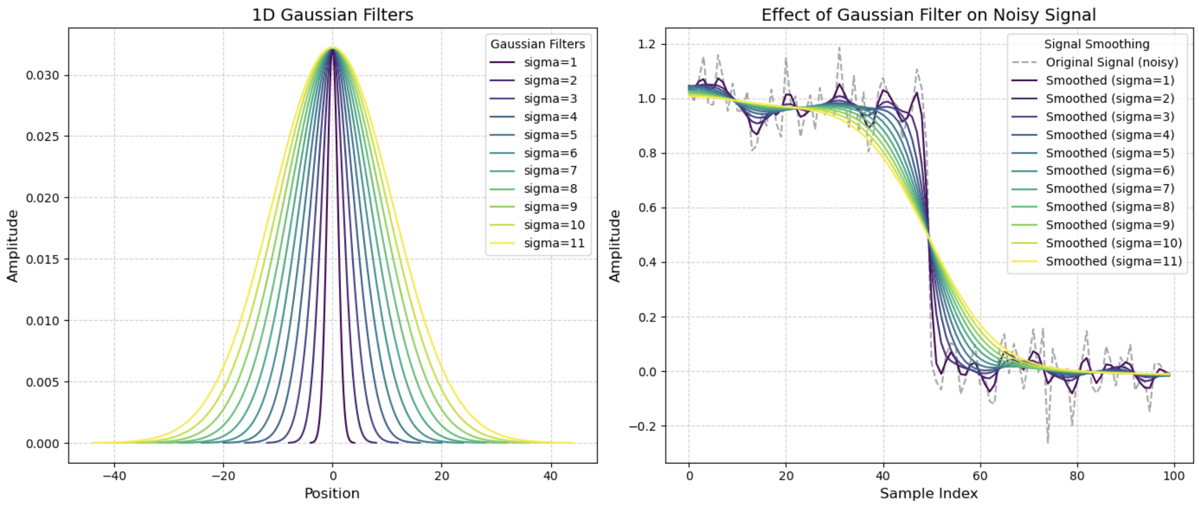
- Task 2: Gaussian filter
- Task 3: Implementing gaussian filter
- Task 4: Reflect on applying gaussian filter
- Task 5: Partial derivatives
- Task 6: Calculate the derivatives
- Task 7: Derivatives of a signal
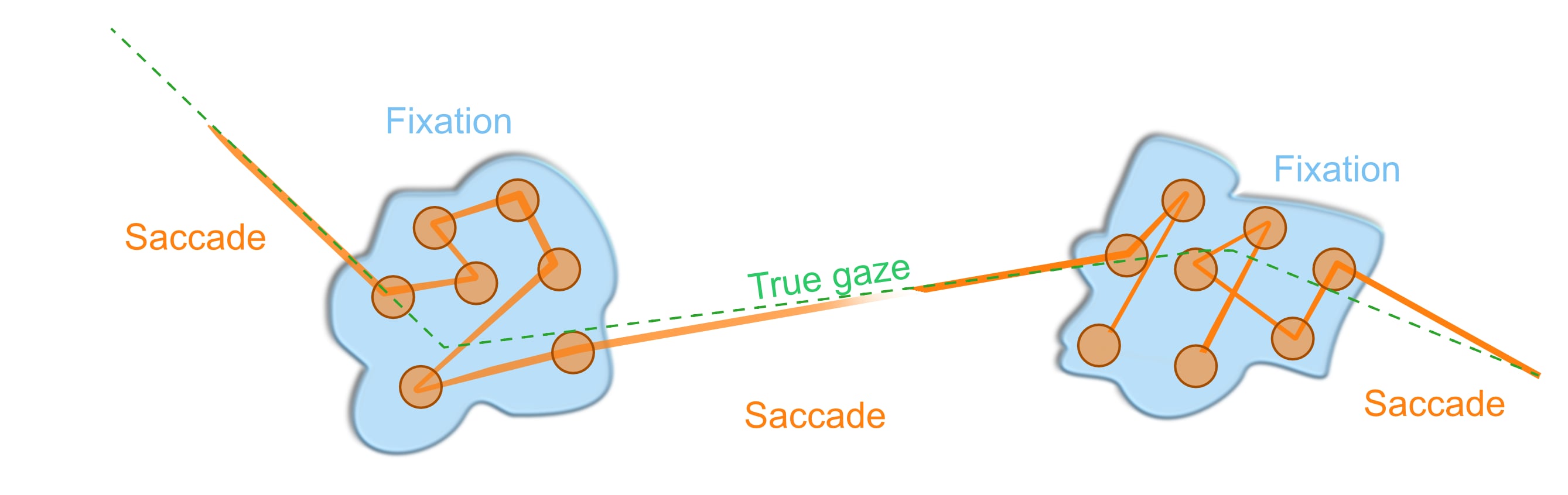
- Task 8: Saccade detection
- Task 9: Saccade detection
- Task 10: Fixation detection
- Task 11: Visualization of signals
- Task 12: Noise handling during fixations
- Task 13: Frame grouping
- Task 14: Analyse results
- Task 15: Reflect
- Task 16: Combined signal
- Task 17: Combined signal
- Task 18: Reflect